Quantum Logic Explorer Home Page

Quantum Logic Explorer    You are about to enter uncharted territory. Unlike elementary Set Theory which is polished and mature mathematics, Quantum Logic is wild and barely explored. An ornery, intractable logic, nobody even knows if it's decidable! (In other words no one knows if an algorithm is even possible that tells you if a given expression is a theorem, much less what such an algorithm might look like.) These pages contain a collection of around 1,000 proofs of my own, my colleague Mladen Pavičić [external], and others. My own proofs are experiments to scout out new terrain, often finding it barren but occasionally stumbling on a small gem or two. All proofs are complete and correct though, verified by the Metamath program with the database file ql.mm.

Credit: Deborah Megill c. 1997. Released to public domain by her estate.

Contents of this page

What is Quantum Logic?

How to Follow Proofs

The Axioms

Some Definitions

Relationship to Hilbert Space

Some Well-Known Theorems

Unifying the Arrow

Weaker Systems

Quantum Propositional Calculus, and a Classical Surprise

Stronger Systems

References

Related pages

Table of Contents and Theorem List

Definition List

Hilbert Space Explorer Home Page

ASCII Equivalents for Text-Only Browsers

What's this? Look for L46-7 at the bottom of this page.

What Is Quantum Logic?    The definition of "quantum logic" varies among authors. What we mean by quantum logic is a Hilbert lattice, which is the set of closed subspaces of an infinite dimensional complex Hilbert space. In particular, we are interested in studying the the set of all equations that hold in this lattice. The subset of these equations that has been studied the most are the equations for orthomodular lattices that we show below. These simple equations can be manipulated with no knowledge of advanced math, and the Quantum Logic Explorer uses them to derive some interesting results worked out in complete detail that anyone with patience can follow.

There are other slightly different, but related, definitions of quantum logic. Some authors use "quantum logics" to mean orthomodular posets [external], whose equations are weaker than those for orthomodular lattices and therefore apply to a larger class of algebras. (An algebra is a set of elements together with operations on those elements. The class of all algebras that obey a given set of equations is called an equational variety.) Other authors mean a propositional calculus based on orthomodular lattices. Below we show how to translate our quantum logic equations to and from this propositional calculus, which is similar to translating the equations for Boolean algebras to and from ordinary classical propositional calculus.

Does quantum logic have anything to do with qubits or quantum computing? The brief answer is "no," and if that's what you are interested in you have probably come to the wrong place. However, there is a connection - our quantum logic, with some additional axioms, determines an infinite dimensional Hilbert space over the field of complex numbers (proved by Maria Solèr in 1995 and refined by René Mayet in 1998 [MegPav2000]). Hilbert space, in turn, provides the theoretical foundation for quantum mechanics and thus quantum computing. But a theory that allows our quantum logic results to be exploited in a practical sense for quantum computing has so far remained an elusive unsolved problem.

Quantum logic together with the additional axioms needed for Solèr's theorem is called the theory of Hilbert lattices. Hilbert lattices and Hilbert space provide dual and equivalent foundations for quantum mechanics, just as the frequency domain and the time domain provide dual descriptions of electrical signals. Just as Fourier transforms have led to greater insight into the nature of electrical signals, it may be possible that, via Solèr's theorem, quantum logic and Hilbert lattices will lead to new results in quantum mechanics. Since Solèr's theorem is so new, very little is known, making the theory of Hilbert lattices an interesting and exciting topic to explore.

How to Follow Proofs    For quantum logic, there is only one type of variable, a term variable (brown color). Simply stated, a proof step results from the substitution of term expressions for the variables in an earlier axiom, definition, or theorem, matching its hypotheses, if any, to either previous steps of the proof or the hypotheses of the theorem being proved. Term expressions are constructed according to the syntax specified in the definition list. To get some practice in following proofs, start with the simple theorems in the Some Well-Known Theorems section below, and this rule should become apparent. It may also be helpful to read the Metamath Proof Explorer's How Proofs Work. The rules are essentially the same those as for the propositional calculus proofs in the Metamath Proof Explorer, except that we use "term" instead of "wff."

The Axioms    Quantum logic can be conveniently broken down into 3 sets of axioms: the ortholattice axioms, the orthomodular law (which holds in those ortholattices that are also orthomodular lattices), and stronger axioms (which hold in those orthomodular lattices that are also Hilbert lattices).

The first two sets of axioms are show below in this section, and the stronger axioms are discussed in the section Stronger Systems below. Whereas the first two sets of axioms have been widely studied, only a few of the stronger axioms, such as the Godowski and orthoarguesian equations discussed below, are known; it is known that they are infinite in number, but it is not known whether they are recursively enumerable.

The theory of ortholattices is decidable, meaning that given any equation, there is an algorithm that will either find a proof for it or show that it is not a theorem. (William McCune wrote a program called olfilter [external] that implements Brun's decision procedure for ortholattices.) It is not known whether the theory of orthomodular lattices, as well as the theories involving the stronger axioms, are decidable, although equations with only two variables are decidable. (The program beran implements the decision procedure for orthomodular lattice equations with two variables. The program lattice is a handy preliminary filter that tests orthomodular lattice conjectures with three or more variables against a collection of useful counterexamples.)

All axioms involve two primitive operations: a negation-like unary postfix operation called orthocomplementation wn (_|_), and an OR-like binary operation called join (or disjunction or supremum) wo (v). (The join should not be confused with the union operation of set theory. The v symbol is a traditional one used in this field.) Formally, an ortholattice or an orthomodular lattice is an algebra <.A, v, _|_>. where A is the base set, v is a binary operation, and _|_ is a unary operation, obeying the axioms below for an ortholattice or orthomodular lattice respectively.

The axioms for an ortholattice are the following equations and inferences. For completeness, we include axioms for equality that are necessary for any algebra. The & and => are informal symbols indicating the relationship between hypotheses and conclusion.

Axioms for an Ortholattice

ax-a1	a = a_|__|_
ax-a2	(a v b) = (b v a)
ax-a3	((a v b) v c) = (a v (b v c))
ax-a4	(a v (b v b_|_)) = (b v b_|_)
ax-a5	(a v (a_|_ v b)_|_) = a
ax-r1	a = b   =>    b = a
ax-r2	a = b   &    b = c   =>    a = c
ax-r4	a = b   =>    a_|_ = b_|_
ax-r5	a = b   =>    (a v c) = (b v c)

To these we add the orthomodular law, which turns the equational system for ortholattices into the stronger equational system for into orthomodular lattices.

Orthomodular Law

ax-r3

(c v c_|_) = ((a_|_ v b_|_)_|_ v (a v b)_|_)    =>    a = b

Some Definitions    Definitions are introduced by connecting, via the equality symbol, a new constant or new term on the left-hand side to the expression it abbreviates on the right-hand side. (In the Metamath language, definitions are introduced in the same way as axioms, with their metalogical soundness justification done outside of the database.)

Some convenient definitions are equivalence (or biconditional or identity), meet (or conjunction or infimum or AND), unit (or true), and zero (or false). Note that the theorem tt justifies our definition of the unit (needed since there is a free variable on the right-hand side that is not on the left-hand side).

Some Definitions

df-b	(a == b) = ((a_|_ v b_|_)_|_ v (a v b)_|_)
df-a	(a ^ b) = (a_|_ v b_|_)_|_
df-t	1 = (a v a_|_)
df-f	0 = 1_|_

With these definitions, the orthomodular law can be rewritten more compactly:

Orthomodular Law

r3a	1 = (a == b)   =>    a = b

For the complete list of syntax and definitions, see the definition list.

Relationship to Hilbert Space    The set of closed subspaces of Hilbert space, CH, determines a special case of an orthomodular lattice <.A, v, _|_>.. Specifically, it is the algebra <.CH, vH, _|_>., where the base set and operations are defined as df-ch, df-chj, and df-oc in the Hilbert Space Explorer, where we prove that the orthomodular lattice axioms above hold for this algebra.

Only relatively recently it was discovered that equations stronger than just the orthomodular lattice axioms hold in this algebra. An important open problem is identifying all such equations.

Some Well-Known Theorems    First we show some simple consequences of the axioms. You may want to study their proofs to become acquainted with the Quantum Logic Explorer's proof notation and to get a feel for the axioms. None of these simple theorems require the use of axiom ax-r3. The list of axioms involved in the proof of each theorem is shown below its proof.

Some Simple Theorems

id	a = a
or1	(a v 1) = 1
an1	(a ^ 1) = a
oridm	(a v a) = a

Any theorem that is equivalent to the orthomodular law axiom ax-r3 (in the presence of the ortholattice axioms) is called an orthomodular law (OM law). Without ax-r3, quantum logic is decidable; with it decidability is unknown. The following version of the OM law, derived using ax-r3, is frequently used.

Orthomodular Law

oml	(a v (a_|_ ^ (a v b))) = (a v b)

An outstanding feature of quantum logic compared to ordinary Boolean algebras is that the distributive law of conjunction (AND) over disjunction (OR) fails, i.e., the system lacks this law. The Foulis-Holland theorems (proved independently by Foulis and Holland) provide weak but very useful versions of the distributive law. The relation "a C b", defined as "a = ((a ^ b) v (a ^ b_|_))", is read "a commutes with b" (see df-c1).

Foulis-Holland Theorems

fh1	a C b   &    a C c   =>    (a ^ (b v c)) = ((a ^ b) v (a ^ c))
fh2	a C b   &    a C c   =>    (b ^ (a v c)) = ((b ^ a) v (b ^ c))
fh3	a C b   &    a C c   =>    (a v (b ^ c)) = ((a v b) ^ (a v c))
fh4	a C b   &    a C c   =>    (b v (a ^ c)) = ((b v a) ^ (b v c))

There are several interesting "exchange theorems" involving the "commutes" relationship. One of them is Gudder-Schelp's Theorem, later strengthened by Beran.

Gudder-Schelp-Beran Theorem

gsth2

b C c   &    a C (b ^ c)   =>    (a ^ b) C c

Another remarkable distributive law was discovered by Marsden and Herman. The hypotheses for this law state that the variables form a commutative "chain."

Marsden-Herman Distributive Law

mh2	a C b   &   b C c   &   c C d   &   d C a   =>    ((a v b) ^ (c v d)) = (((a ^ c) v (a ^ d)) v ((b ^ c) v (b ^ d)))

One consequence of the Marsden-Herman law is the following interesting distributive law involving the biconditional. Previously it was known only that this law followed from the stronger Godowski equations [MegPav2001]; here we show a new proof [MegPav2003a] that requires only the axioms for orthomodular lattices.

Distributive Law for Biconditional

distid

((a == b) ^ ((a == c) v (b == c))) = (((a == b) ^ (a == c)) v ((a == b) ^ (b == c)))

The complete list of theorems in the Quantum Logic Explorer database is provided by the theorem list.

Unifying the Arrow    The "natural" primitives of quantum logic are conjunction, disjunction, and negation. There are five possibilities for definining implication in quantum logic in terms of them: Sasaki (df-i1), Dishkant (df-i2), Kalmbach (df-i3), non-tollens (df-i4), and relevance (df-i5). It has been shown that these are the only possibilities that satisfy an important ordering relationship known as the Birkhoff-von Neumann requirement. In a Boolean algebra, these all reduce to classical implication (a_|_ v b) (df-i0).

The Five Quantum Implications

df-i1	(a ->1 b) = (a_|_ v (a ^ b))
df-i2	(a ->2 b) = (b v (a_|_ ^ b_|_))
df-i3	(a ->3 b) = (((a_|_ ^ b) v (a_|_ ^ b_|_)) v (a ^ (a_|_ v b)))
df-i4	(a ->4 b) = (((a ^ b) v (a_|_ ^ b)) v ((a_|_ v b) ^ b_|_))
df-i5	(a ->5 b) = (((a ^ b) v (a_|_ ^ b)) v (a_|_ ^ b_|_))

Attempts to justify the "true" implication has been a topic of much investigation and philosophical debate. So we were surprised to discover [PavMeg1998b] that they can all be unified into one, allowing a quantum logic axiom system to be devised with a "universal" implication (which could be any one of the five) and negation as the only primitives.

The way this is done is as follows. We show that disjunction is equivalent to (and thus can be defined by) a structural formula with an arbitrary implicational connective that could be any one of the five. We then use this formula for disjunction to replace the disjunction symbol in a formulation (axiom system) of quantum logic with disjunction and negation as the only primitives. This gives us an axiom system with only implication and negation as the only primitives, where the implication can be any one of the five.

Here are the structurally identical formulas for disjunction in terms of implication. Pretty neat, don't you think? Their proofs are quite tedious, though - take a peek at them.

Disjunction in Terms of the Five Implications

ud1	(a v b) = ((a ->1 b) ->1 (((a ->1 b) ->1 (b ->1 a)) ->1 a))
ud2	(a v b) = ((a ->2 b) ->2 (((a ->2 b) ->2 (b ->2 a)) ->2 a))
ud3	(a v b) = ((a ->3 b) ->3 (((a ->3 b) ->3 (b ->3 a)) ->3 a))
ud4	(a v b) = ((a ->4 b) ->4 (((a ->4 b) ->4 (b ->4 a)) ->4 a))
ud5	(a v b) = ((a ->5 b) ->5 (((a ->5 b) ->5 (b ->5 a)) ->5 a))

Weaker Systems    An interesting system to study is one in which an orthomodular lattice's ax-r3 is replaced by a weaker axiom called the weakly orthomodular (WOM) law [PavMeg1998a]. We show three equivalent forms below. In the Quantum Logic Explorer database we have called the first one an axiom, and the other two are derived from it using only the axioms for ortholattices (look at the line called "The theorem was proved from these axioms" at the end of each proof listing, and there will be no mention of ax-r3). In [PavMeg1998a] we show that ax-wom is strictly weaker than ax-r3.

Weakly Orthomodular Law Equivalents

ax-wom	(a_|_ v (a ^ b)) = 1   =>    (b v (a_|_ ^ b_|_)) = 1
woml6	((a ->1 b)_|_ v (a ->2 b)) = 1
ka4ot	((a == b)_|_ v ((a v c) == (b v c))) = 1

In a WOM system we can prove a set of theorems that are isomorphic to (structurally resemble) the axioms and rules of orthomodular lattices. The analogous theorem is created by replacing "=" with "==" in an orthomodular lattice theorem, then suffixing it with "= 1". This means that the axiom system for for orthomodular lattices can effectively be embedded in a strictly weaker subset of itself! In particular, decidability of the weaker system implies decidability of the stronger one and vice-versa. (The decision problem is one of the most important unsolved problems in quantum logic.) Counterintuitively, wr3, which is the structural analog for the orthomodular law ax-r3, can be proved with only the ortholattice axioms and does not require even the WOM law (whereas ax-r3 is the OM law). However, the structural analogs for an ortholattice's ax-r2 and ax-r5 (which are really nothing more than equality laws holding in any algebra) do require the WOM law. In each particular case, the axioms used for the proof are shown below the proof in the page referenced by the hyperlink; note that ax-r3 is not used for any of them.

Weakly Orthomodular Structural Analogs for Orthomodular Lattice Axioms

wa1	(a == a_|__|_) = 1
wa2	((a v b) == (b v a)) = 1
wa3	(((a v b) v c) == (a v (b v c))) = 1
wa4	((a v (b v b_|_)) == (b v b_|_)) = 1
wa5	((a v (a_|_ v b_|_)_|_) == a) = 1
wr1	(a == b) = 1   =>    (b == a) = 1
wr2	(a == b) = 1   &    (b == c) = 1   =>    (a == c) = 1
wr3	(1 == a) = 1   =>    a = 1
wr4	(a == b) = 1   =>    (a_|_ == b_|_) = 1
wr5	(a == b) = 1   =>    ((a v c) == (b v c)) = 1

These structural analogs to the orthomodular lattice axioms come in handy for proving various properties of weakly orthomodular systems. We can prove a theorem in the normal way with the standard axioms, then mimic the proof with the structural analogs above to obtain the weakly orthomodular analog. For example, we can derive weakly orthomodular analogs of the Foulis-Holland theorems: wfh1, wfh2, wfh3, and wfh4. Note that for each of these, ax-r3 is never required for the proof, but only ax-wom.

A very interesting result [PavMeg1998a] is that we can derive the structural analog of the OM law oml without referring even to ax-wom! In the past it seems it was believed that this law supplied the orthomodular property for quantum propositional calculus axiomatizations called "unary logics," but instead it turns out to be a law of pure ortholattice theory. Thus we call it the "faux orthomodular law." In fact, the (weakly) orthomodular property for such logics is hidden in the innocent-looking wr5, which has the appearance of a simple equality axiom. Such are the surprises to be found in quantum logic.

Faux orthomodular law

woml	((a v (a_|_ ^ (a v b))) == (a v b)) = 1

Quantum Propositional Calculus    Quantum logic is often expressed and studied as a propositional calculus. Just as classical propositional calculus is based on Boolean algebras, quantum propositional calculus is based on orthomodular lattices. Going from the lattice equations to the propositional calculus is completely analogous to the classical case: any equality whose right-hand side is 1 (this is called a valuation) corresponds to the proposition with the right-hand side removed. (Technically, this is called a unary propositional calculus). Thus, for example, the law of excluded middle (a v a_|_) = 1 (which is a theorem of quantum logic that follows from tt and df-t) corresponds to the proposition "A \/ -.A" (where A is a wff, or propositional, variable). Thus each of the WOM structural analogs for the orthomodular lattice axioms, shown in the previous section, corresponds to a statement of quantum propositional calculus; in fact these are the exact axioms of quantum propositional calculus.

Lattice O6 What is particularly interesting is that quantum propositional calculus can be modeled by any WOM lattice. The class of WOM lattices includes all orthomodular lattices but some non-orthomodular ones as well. For example, a hexagonal-shaped WOM lattice called O6 is non-orthomodular, but is still a model for quantum propositional calculus. This apparently was not known prior to 1998 [PavMeg1998a] [PavMeg1999].

Quantum propositional calculus can be formalized with modus ponens as its sole rule of inference,and negation and implication as its sole primitive connectives, as long as we use for the implication either ->0 (wi0) or ->3 (wi3). Kalmbach proved that these are the only two implications that work. We prove soundness for her axiom system as theorems ska1, ska2 (500K), ska3, ska4, ska5, ska6, ska7, ska8, ska9, ska10, ska11, ska12, ska13, ska14, ska15, and (for the two possible rules) skr0 and skmp3. In the soundness proofs, we never use the orthomodular law ax-r3, but only the weaker WOM law ax-wom, so these theorems provide a rigorous proof that the full strength of orthomodular lattice theory is not needed for quantum propositional calculus.

Classical propositional calculus has non-Boolean lattice models     Related to this and even more surprising is that classical propositional calculus can be modeled by a non-Boolean lattice [PavMeg1999], a fact apparently overlooked for over 100 years! Common intuition is that classical propositional calculus and Boolean algebras go hand-in-hand. Lattice O6 is a counterexample that shows this intuition is false. Specifically, lattice O6 is a model for classical propositional calculus, but it violates the axioms for Boolean algebras (the distributive law fails). This is proved as follows. If we define a->b as a_|_vb, then the 3 axioms of classical propositional calculus evaluate to 1 (true), and modus ponens is sound. So O6 is a model for classical propositional calculus. However, the distributive law x^(yvz)=(x^y)v(x^z) fails in this lattice: Let x=a, y=b, z=b_|_. Then x^(yvz)=a^(bvb_|_)=a^1=a, but (x^y)v(x^z)=(a^b)v(a^b_|_)=bv0=b. Therefore lattice O6 is a non-distributive model for classical propositional calculus.

More generally, classical propositional calculus can be modelled by a class of algebras known as "weakly distributive ortholattices" (WDOLs), which in general are non-Boolean. In particular, O6 is a WDOL. The WDOL axiom (which when added to an ortholattice, provides an equational base for WDOLs) is ax-wdol. The theorems from there to the end of the database are currently (as of 16-Mar-2006) WDOL theorems.

Stronger Systems    The motivation for studying quantum logic (and the related orthomodular lattices) derives from the fact that the lattice of closed subspaces of a Hilbert space, called CH, obeys the properties of an orthomodular lattice (see Quantum Logic on the Hilbert Space Explorer Home Page). Hilbert space underlies the foundation of quantum mechanics, and there is a strong physical and philosophical motivation to understand its properties. In addition, understanding the properties of Hilbert space is important for understanding what kinds of operations are possible in the new field of quantum computers.

It turns out that Hilbert space obeys not only the equations of orthomodular lattices but some stronger equations as well. This was not known until 1975, when Alan Day discovered the "orthoarguesian law," an equation closely related to a famous law of projective geometry discovered by Desargues in the 1600's as part of an effort to help artists, stonecutters, and engineers.

The orthoarguesian (4OA) law can be added as an additional axiom to orthomodular lattices to obtain an axiom system that is stronger than that for orthomodular lattices but still true in CH. This axiom system is still weaker than that for Boolean algebras because the distributive law does not hold, so the resulting axioms fall somewhere between those for orthomodular lattices and those for Boolean algebras. We have studied the 4-variable 4OA law as well as a weaker 3-variable consequence called 3OA [MegPav2000]. The 3OA law was originally found by Godowski and Greechie and is easier to work with. Many of the properties of 3OA can be easily generalized to 4OA, and that is one of the reasons to investigate 3OA as well as the more general 4OA. (See wle for the notation "=<".)

3OA Law and 4OA (Orthoarguesian) Law

ax-3oa	((a ->1 c) ^ ((a ^ b) v ((a ->1 c) ^ (b ->1 c)))) =< (b ->1 c)
ax-4oa	((a ->1 d) ^ (((a ^ b) v ((a ->1 d) ^ (b ->1 d))) v (((a ^ c) v ((a ->1 d) ^ (c ->1 d))) ^ ((b ^ c) v ((b ->1 d) ^ (c ->1 d)))))) =< (b ->1 d)

The original discovery of Alan Day was an inference rule involving 6 variables. Our 4OA equation is equivalent to it in the presence of the orthomodular lattice axioms. Below we show the original orthoarguesian law as a theorem derived from 4OA.

Original 6-variable Orthoarguesian Law

oa6	a =< b_|_   &    c =< d_|_   &    e =< f_|_   =>    (((a v b) ^ (c v d)) ^ (e v f)) =< (b v (a ^ (c v (((a v c) ^ (b v d)) ^ (((a v e) ^ (b v f)) v ((c v e) ^ (d v f)))))))

Using the orthoarguesian law we can derive distributive laws that are stronger than those provided by the Foulis-Holland theorems. Below we show two of them, derived respectively from 3OA and 4OA. In fact, they can be shown to be equivalent to 3OA and 4OA respectively. Theorem d4oa, not shown here, derives 4OA from the second distributive law below. (See wi0 for the notation "->0".) While the hypotheses for these laws are complex and non-intuitive, look at the conclusion - there you will see the distributive law.

3OA and 4OA Distributive Laws

oadistd	d =< (a ->2 b)   &    e =< ((b v c) ->0 ((a ->2 b) ^ (a ->2 c)))   &    f =< ((b v c) ->0 ((a ->2 b) ^ (a ->2 c)))   &    (d ^ (a ->2 c)) =< f   =>    (d ^ (e v f)) = ((d ^ e) v (d ^ f))
4oadist	e = (((a ^ c) v ((a ->1 d) ^ (c ->1 d))) ^ ((b ^ c) v ((b ->1 d) ^ (c ->1 d))))   &    f = (((a ^ b) v ((a ->1 d) ^ (b ->1 d))) v e)   &    h =< (a ->1 d)   &    j =< f   &    k =< f   &    (h ^ (b ->1 d)) =< k   =>    (h ^ (j v k)) = ((h ^ j) v (h ^ k))

Recently [MegPav2000] we found an infinite series of even stronger orthoarguesian-like laws that hold in Hilbert space, that we call 5OA, 6OA, 7OA... with 5, 6, 7... variables. We proved that 5OA is strictly stronger than 4OA [MegPav2000] and more recently that 6OA is strictly stronger than 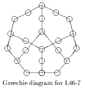5OA and that 7OA is strictly stronger than 6OA (a task that took many CPU years of computer time on a supercomputer cluster). The status of the higher-order ones is unknown but they are conjectured to be even stronger.

There are currently no theorems involving 5OA and up in the Quantum Logic Explorer, but a proof that 5OA holds in Hilbert space is shown in the Hilbert Space Explorer. A proof that 5OA is strictly stronger than 4OA is provided by orthomodular lattice L46-7 (found by our computer search), shown in the form of a "Greechie diagram" in the figure. Lattice L46-7 provides a counterexample that holds in 4OA but not in 5OA. (Greechie diagrams provide a compact way of representing orthomodular lattices. Reference 9, PDF file p. 13 has a tutorial explaining how they correspond to lattices. The Greechie diagram for L46-7 represents a 46-node lattice.)

As n increases, the formula for nOA grows quite long and is inconvenient to work with directly. In the box below we show an abbreviated notation for nOA used in Reference 7.

nOA equation definition

Another set of stronger equations that hold in Hilbert space is derived from the properties strong states on a Hilbert lattice. One family of these was discovered by Godowski in 1981. The simplest one is the 3-variable Godowski equation. In the Quantum Logic Explorer, we prove that two equations from the literature, gomaex3 and gomaex4, apparently believed to be independent of Godowki's, in fact follow from them [MegPav2000]. Recently we found a series of new equations related to strong states, holding in the set of closed subspaces of Hilbert space, that are independent from Godowski's. These have not been published yet. The simplest one is shown below.

(((a ->1 b) ->1 (c ->1 b)) ^ ((a ->1 c) ^ (b ->1 a))) =< (c ->1 a)

References   

(See also the References for the Hilbert Space Explorer.)

1. [Kalmbach] Gudrun Kalmbach, Orthomodular Lattices, Academic Press, London (1983).
2. [Beran] Ladislav Beran, Orthomodular Lattices; Algebraic Approach, D. Reidel, Dordrecht (1985).
3. [Pavicic1987] M. Pavičić, "Minimal Quantum Logic with Merged Implications," Int. J. of Theor. Phys. 26, 845-852 (1987).
4. [Pavicic1993] M. Pavičić, "Nonordered Quantum Logic," Int. J. of Theor. Phys. 32, 1481-1505 (1993), http://m3k.grad.hr/papers-ps-pdf/quantum-logic/1993-int-j-theor-phys-2.pdf [external].
5. [PavMeg1998a] M. Pavičić and N. Megill, "Binary Orthologic with Modus Ponens Is either Orthomodular or Distributive," Helv. Phys. Acta 71, 610-628 (1998), http://m3k.grad.hr/papers-ps-pdf/quantum-logic/1998-helv-phys-acta.pdf [external].
6. [PavMeg1998b] M. Pavičić and N. Megill, "Quantum and Classical Implicational Algebras with Primitive Implication," Int. J. of Theor. Phys. 37, 2091-2098 (1998), http://m3k.grad.hr/papers-ps-pdf/quantum-logic/1998-int-j-theor-phys-2.pdf [external].
7. [PavMeg1999] M. Pavičić and N. Megill, "Non-Orthomodular Models for Both Standard Quantum Logic and Standard Classical Logic: Repercussions for Quantum Computers," Helv. Phys. Acta 72, 189-210 (1999), http://xxx.lanl.gov/abs/quant-ph/9906101 [external].
8. [MegPav2000] N. Megill and M. Pavičić, "Equations, States, and Lattices of Infinite-Dimensional Hilbert Space," Int. J. Theor. Phys. 39, 2337-2379 (2000), http://xxx.lanl.gov/abs/quant-ph/0009038 [external].
9. [McKMegPav] B. McKay, N. Megill, and M. Pavičić, "Algorithms for Greechie Diagrams," Int. J. Theor. Phys. 39, 2393-2417 (2000), http://xxx.lanl.gov/abs/quant-ph/0009039 [external].
10. [MegPav2001] N. Megill and M. Pavičić, "Orthomodular Lattices and a Quantum Algebra," Int. J. Theor. Phys. 40, 1387-1410 (2001), http://xxx.lanl.gov/abs/quant-ph/0103135 [external].
11. [MegPav2002] N. Megill and M. Pavičić "Deduction, ordering, and operations in quantum logic," Found. Phys. 32, 357-378 (2002), http://xxx.lanl.gov/abs/quant-ph/0108074 [external].
12. [MegPav2003a] N. Megill and M. Pavičić, "Equivalences, Identities, Symmetric Differences, and Congruences in Orthomodular Lattices," Int. J. Theor. Phys. 42, 2797-2805 (2003), http://xxx.lanl.gov/abs/quant-ph/0310063 [external].
13. [MegPav2003b] N. Megill and M. Pavičić, "Quantum Implication Algebras," Int. J. Theor. Phys. 42, 2807-2822 (2003), http://xxx.lanl.gov/abs/quant-ph/0310062 [external].
14. [PavMerMcKMeg] M. Pavičić, J.-P. Merlet, B. McKay, and N. Megill, "Kochen-Specker Vectors," preprint (2004), http://arxiv.org/quant-ph/0409014 [external].

Note: For on-line copies of some of these and other quantum logic papers, visit the Home Page of Mladen Pavičić [external].