Hilbert Space Explorer Home Page

Hilbert Space Explorer   

Hilbert space (Wikipedia [external], MathWorld [external]) is a generalization of finite-dimensional vector spaces to include vector spaces with infinite dimensions. It provides a foundation of quantum mechanics, and there is a strong physical and philosophical motivation to study its properties. For example, the properties of Hilbert space ultimately determine what kinds of operations are theoretically possible in quantum computation.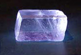

Calcite

Contents of this page How to Follow the Proofs Symbol List Two Approaches to Hilbert Space The Axioms Revised 10-Sep-2009 Some Definitions Some Theorems Quantum Logic What Next? (Orthoarguesian Law, etc.) References

Related pages Table of Contents and Theorem List Bibliographic Cross-Reference Metamath Proof Explorer Home Page Quantum Logic Explorer Home Page

How to Follow the Proofs    We develop Hilbert space theory as an extension of ZFC set theory, and many steps in various proofs use results from set theory. To understand how to read the proofs, see How Proofs Work on the Metamath Proof Explorer Home Page. Symbol List    The chart below provides a quick reference for the new symbols introduced in the Hilbert Space Explorer. The five symbols marked "primitive" are postulated to have the properties specified by the axioms, and the rest are defined in terms of them. The complete list of all syntax elements, axioms, and definitions used by the Hilbert Space Explorer pages, including those for the underlying logic and ZFC set theory, is provided in the Definition List (900K).

Symbol List for Hilbert Space

Symbol	Description	Link to Definition
H~	Hilbert space base set	(primitive)
+h	vector addition	(primitive)
.s	scalar multiplication	(primitive)
0h	zero vector	(primitive)
.ih	inner (scalar) product	(primitive)
-h	vector subtraction	df-hvsub
normh	norm of a vector	df-hnorm
Cauchy	set of Cauchy sequences	df-hcau
~~>v	convergence relation	df-hlim
SH	set of subspaces	df-sh
CH	set of closed subspaces	df-ch
_|_	orthocomplement	df-oc
+H	subspace sum	df-shs
span	subspace span	df-span
vH	join	df-chj
\/H	supremum	df-chsup
0H	zero subspace	df-ch0
C_H	commutes relation	df-cm
+op	operator sum; definition of "operator"	df-hosum
.op	operator scalar product	df-homul
-op	operator difference	df-hodif
+fn	functional sum; definition of "functional"	df-hfsum
.fn	functional scalar product	df-hfmul
0hop	zero operator	df-h0op
iop	identity operator	df-iop
proj	projection operator (projector)	df-pj
normop	norm of an operator	df-nmop
ConOp	set of continuous operators	df-cnop
LinOp	set of linear operators	df-lnop
BndLinOp	set of bounded linear operators	df-bdop
UniOp	set of unitary operators	df-unop
HrmOp	set of Hermitian operators	df-hmop
normfn	norm of a functional	df-nmfn
null	null space of a functional	df-nlfn
ConFn	set of continuous functionals	df-cnfn
LinFn	set of linear functionals	df-lnfn
adjh	adjoint of an operator	df-adjh
bra	Dirac "bra" of a vector	df-bra
<_op	ordering relation for positive operators	df-leop
ketbra	Dirac "ket-bra" (outer product) of two vectors	df-kb
eigvec	eigenvectors of an operator	df-eigvec
eigval	eigenvalue of an eigenvector	df-eigval
Lambda	spectrum of an operator	df-spec
States	set of states	df-st
CHStates	set of (Mayet's) Hilbert-space-valued states	df-hst
Atoms	set of atoms	df-at
<o	covering relation	df-cv
MH	modular pair relation	df-md
MH*	dual modular pair relation	df-dmd

Two Approaches to Hilbert Space    There are several ways to develop the theory of Hilbert spaces. The purest way, philosophically, is to define the class of all Hilbert spaces and use only the axioms of ZFC set theory to derive its properties. That way we need to assume only the axioms of ZFC (which in principle is all that is needed for essentially all of mathematics, including the theory of Hilbert spaces). This is done in the Metamath Proof Explorer with definition df-hl.

However, we chose separate axioms for the Hilbert Space Explorer for several reasons. A practical problem with the pure ZFC approach is that theorems becomes somewhat awkward to state and prove, since they usually need additional hypotheses. Compare, for example, the ZFC-derived hlcom with the Hilbert Space Explorer axiom ax-hvcom. Another advantage for a newcomer is that the Hilbert Space Explorer states outright all of its axioms, so there is nothing else to learn (aside from standard set theory tools to manipulate them). In the Metamath Proof Explorer, on the other hand, one needs to become familiar with the hierarchy of groups, topologies, vector spaces, metric spaces, normed vector spaces, and Banach spaces that leads to Hilbert spaces.

If we want to use the Hilbert Space Explorer with any fixed Hilbert space, such as the set of complex numbers (which, as it turns out, is an example of a Hilbert space - see theorem cnhl), a simple change to the axiomatization will convert all theorems in the Hilbert Space Explorer to pure ZFC theorems. A description of how this can be done is given in the comment for axiom ax-hilex. On the other hand, if we want to prove theorems involving relationships between Hilbert spaces, the Hilbert Space Explorer may not be not suitable, but rewriting its proofs for the general ZFC approach as needed is relatively straightforward. (Actually, many such theorems can still be done in the Hilbert Space Explorer itself using subspaces, each of which acts like a stand-alone Hilbert Space.)

The Axioms    In our separately axiomatized approach of the Hilbert Space Explorer, we postulate the existence of a new primitive fixed object, H~ (chil), called the Hilbert space base set, and add to ZFC set theory explicit axioms for the properties of H~. The members of H~ are called vectors, and they have the same properties as the vectors you normally find in any linear algebra textbook, except that the dimension (the number of basis vectors) is not specified and may be infinite. In addition to H~, we postulate the existence and properties of 4 more objects: a fixed zero vector 0h (c0v); the operations of vector addition +h (cva) and scalar multiplication .h (csm); and finally, an inner product operation .ih (csp). The five objects H~, 0h, +h, .h, and .ih are the complete set of objects needed to describe Hilbert space. We will encounter other objects as well, but all of them are defined either in terms of these five, or as specific sets of set theory. For example, the object CC (the set of complex numbers cc) is defined as a specific set of set theory.

The page for each axiom below is accompanied by a precise breakdown of its syntax. You can break the syntax down into as much detail as you want by using the hyperlinks in the syntax breakdown chart. Note our use of the notation "(A .ih B)" instead of the more common notation "<.A,B>." for inner products; the latter would conflict with our notation for ordered pairs cop.

Axioms for Hilbert Space

ax-hilex	|- H~ e. V
ax-hfvadd	|- +h :(H~ X. H~)-->H~
ax-hvcom	|- ((A e. H~ /\ B e. H~) -> (A +h B) = (B +h A))
ax-hvass	|- ((A e. H~ /\ B e. H~ /\ C e. H~) -> ((A +h B) +h C) = (A +h (B +h C)))
ax-hv0cl	|- 0h e. H~
ax-hvaddid	|- (A e. H~ -> (A +h 0h) = A)
ax-hfvmul	|- .h :(CC X. H~)-->H~
ax-hvmulid	|- (A e. H~ -> (1 .h A) = A)
ax-hvmulass	|- ((A e. CC /\ B e. CC /\ C e. H~) -> ((A x. B) .h C) = (A .h (B .h C)))
ax-hvdistr1	|- ((A e. CC /\ B e. H~ /\ C e. H~) -> (A .h (B +h C)) = ((A .h B) +h (A .h C)))
ax-hvdistr2	|- ((A e. CC /\ B e. CC /\ C e. H~) -> ((A + B) .h C) = ((A .h C) +h (B .h C)))
ax-hvmul0	|- (A e. H~ -> (0 .h A) = 0h)
ax-hfi	|- .ih :(H~ X. H~)-->CC
ax-his1	|- ((A e. H~ /\ B e. H~) -> (A .ih B) = (*`(B .ih A)))
ax-his2	|- ((A e. H~ /\ B e. H~ /\ C e. H~) -> ((A +h B) .ih C) = ((A .ih C) + (B .ih C)))
ax-his3	|- ((A e. CC /\ B e. H~ /\ C e. H~) -> ((A .h B) .ih C) = (A x. (B .ih C)))
ax-his4	|- ((A e. H~ /\ A =/= 0h) -> 0 < (A .ih A))
ax-hcompl	|- (F e. Cauchy -> E.x e. H~F ~~>v x)

Comments on the axioms. The first axiom just says that the primitive class H~ exists (is a member of the universe of sets V). The next 11 axioms are the axioms for any vector space with an unspecified dimension; they are the same as those you would find in any linear algebra book, except for the notation and possibly their precise form.

The next 5 axioms show the properties of the special inner product .ih. The official name for this inner product is a "sesquilinear Hermitian mapping". (Sesquilinear means "one-and-a-half linear," i.e., antilinear in the first argument and linear in the second.) The symbol * in Axiom ax-his1 is the complex conjugate (cjval). See Notation for Function Values for an explanation of why we use this notation rather than the standard superscript asterisk used in textbooks; this will help you understand some of our other non-standard notation as well.

The last axiom, which is the most important and also the most complicated, is called the Completeness Axiom, and is shown above using abbreviations. You can click on its links to expand the abbreviations. It basically says that the limit of any converging ("Cauchy") sequence of vectors in Hilbert space converges to a vector in Hilbert space. To understand what completeness means, consider this analogy: the sequence 3, 3.1, 3.14, 3.1415, 3.14159... converges to pi. This is a converging sequence of rational numbers, but it converges to something that is not a rational number, meaning the set of rational numbers is not complete. The set of real numbers, on the other hand, is complete, because all converging sequences of real numbers converge to a real number.

Some Definitions    Here we show explicitly a few of the definitions you will encounter in our Hilbert space proofs. The complete list is given at the top of this page. We typically define new symbols as a self-contained objects, which can make their definitions seem unnecessarily complicated, but usually their Descriptions point to simpler theorems showing their values or other properties. For example, the vector subtraction operation -h is formally a set of ordered pairs as shown below, but its value is just A +h (-u1 .h B) as can be seen from theorem hvsubval.

Some Definitions for Hilbert Space

The vector subtraction operation df-hvsub	|- -h = {<.<.x,y>.,z>. | ((x e. H~ /\ y e. H~) /\ z = (x +h (-u1 .h y)))}
The norm of a vector df-hnorm	|- normh = {<.x,y>. | (x e. H~ /\ y = (sqrt`(x .ih x)))}
The set of all Cauchy sequences df-hcau	|- Cauchy = {f | (f:NN-->H~ /\ A.x e. RR(0 < x -> E.y e. NNA.z e. NNA.w e. NN((y <_ z /\ y <_ w) -> (normh`((F`z) -h (F`w))) < x)))}
The limit of a vector sequence df-hlim	|- ~~>v = {<.f,w>. | ((f:NN-->H~ /\ w e. H~) /\ A.x e. RR(0 < x -> E.y e. NNA.z e. NN(y <_ z -> (normh`((f`z) -h w)) < x)))}
The set of all subspaces of Hilbert space df-sh	|- SH = {h | ((h (_ H~ /\ 0h e. h) /\ (A.x e. hA.y e. h(x +h y) e. h /\ A.x e. CCA.y e. h(x .h y) e. h))}
The set of all closed subspaces of Hilbert space df-ch	|- CH = {h | (h e. SH /\ A.fA.x((f:NN-->h /\ f ~~>v x) -> x e. h))}
The sum of two subspaces df-shsum	|- +H = {<.<.x,y>.,z>. | ((x e. SH /\ y e. SH) /\ z = {w e. H~ | E.v e. xE.u e. yw = (v +h u)})}

Some Theorems    First we show some basic properties of vectors. These are laws in any vector space, not just Hilbert spaces, so they should be familiar if you've taken a linear algebra course.

Some Basic Properties of Vectors

hvsubcl	|- ((A e. H~ /\ B e. H~) -> (A -h B) e. H~)
hvnegid	|- A e. H~   =>    |- (A +h (-u1 .h A)) = 0h
hvmul0	|- (A e. CC -> (A .h 0h) = 0h)
hvsubid	|- (A e. H~ -> (A -h A) = 0h)
hvsubeq0	|- A e. H~   &   |- B e. H~   =>    |- ((A -h B) = 0h <-> A = B)

Next we show some basic properties of the special inner product defined for Hilbert space.

Theorems Involving Inner Product

his5	|- ((A e. CC /\ B e. H~ /\ C e. H~) -> (B .ih (A .h C)) = ((*`A) x. (B .ih C)))
his6	|- (A e. H~ -> ((A .ih A) = 0 <-> A = 0h))
his7	|- ((A e. H~ /\ B e. H~ /\ C e. H~) -> (A .ih (B +h C)) = ((A .ih B) + (A .ih C)))

Next we show some theorems involving norms. Note our use of the notation "(normh`A)" instead of the more common notation "||A||" - see Notation for Function Values.

Theorems norm-i, norm-ii (triangle inequality), and norm-iii show that the basic properties expected of any norm hold for the norm we defined for Hilbert space. Theorem normpyth is an analogy to the Pythagorean theorem, and theorem normpar is the parallellogram law. Theorem bcs is the Bunjakovaskij-Cauchy-Schwarz inequality.

Theorems Involving Norms

norm-i	|- A e. H~   =>    |- ((normh`A) = 0 <-> A = 0h)
norm-ii	|- A e. H~   &   |- B e. H~   =>    |- (normh`(A +h B)) <_ ((normh`A) + (normh`B))
norm-iii	|- A e. CC   &   |- B e. H~   =>    |- (normh`(A .h B)) = ((abs`A) x. (normh`B))
normpyth	|- A e. H~   &   |- B e. H~   =>    |- ((A .ih B) = 0 -> ((normh`(A +h B))^2) = (((normh`A)^2) + ((normh`B)^2)))
normpar	|- A e. H~   &   |- B e. H~   =>    |- (((normh`(A -h B))^2) + ((normh`(A +h B))^2)) = ((2 x. ((normh`A)^2)) + (2 x. ((normh`B)^2)))
bcs	|- A e. H~   &   |- B e. H~   =>    |- (abs`(A .ih B)) <_ ((normh`A) x. (normh`B))

Next we show some basic theorems about sequences. Theorem hlimcaui shows any converging sequence is a Cauchy sequence and hlimunii shows that the limit of a converging sequence is unique. The theorem pjth is the important Projection Theorem; it shows any vector can be decomposed into a pair of "projections" on a subspace and the orthocomplement of the subspace (see below for the definition of the orthocomplement _|_).

Theorems Involving Limits and Subspaces

hlimcaui	|- A e. V   &   |- F e. V   =>    |- (F ~~>v A -> F e. Cauchy)
hlimunii	|- A e. V   &   |- B e. V   &   |- F e. V   =>    |- ((F ~~>v A /\ F ~~>v B) -> A = B)
pjth	|- A e. H~   &   |- H e. CH   =>    |- E.x e. HE.y e. (_|_`H) A = (x +h y)

Quantum Logic   

The set of closed subspaces of Hilbert space obey the laws of a simple equational algebra called "orthomodular lattice algebra." This algebra is sometimes called "quantum logic," and it can be used as the basis for a propositional calculus that resembles but is somewhat weaker than standard (classical) propositional calculus. This is explained in greater detail in the Quantum Logic Explorer. Our purpose here is to show that the orthomodular lattice laws hold in Hilbert space. This provides a rigorous justification for the axioms of the Quantum Logic Explorer. (By the way, theorem nonbooli shows why classical logic, i.e. Boolean algebra, does not hold in Hilbert space.)

The advantage of the Quantum Logic Explorer is that it lets us work with a simpler axiomatic structure. But in principle, all the theorems of the Quantum Logic Explorer could be proved directly in Hilbert space, using the theorems below as the starting point. In fact in a few cases we do this, because sometimes we need the Hilbert space version to help prove theorems that exploit Hilbert space properties beyond those provided by the orthomodular lattice laws alone. For example, compare the proofs of the Hilbert Space Explorer theorem fh3i and the Quantum Logic Explorer version fh3. If you ignore the steps with an "e." in the Hilbert space version, you'll see the proofs are almost identical except for notation; in fact, any differences beyond that just result from the proofs having been developed somewhat independently. You can see why the Quantum Logic Explorer is simpler to work with for these kinds of things: we don't need the "e. CH" hypotheses, and we don't have to keep proving operation closure over and over.

To derive the orthomodular lattice postulates, first we define two new operations on members of CH (the set of closed subspaces of Hilbert space). The orthocomplement of a subspace is the set of vectors orthogonal to all vectors in the subpace. It is analogous to logical NOT. The join of two subspaces is the closure (i.e. the double orthocomplement) of their union. It is analogous to logical OR.

Lattice Definitions for CH

Orthocomplement chocvali	|- A e. CH   =>   |- (_|_` A) = {x e. H~ | A.y e. A (x .ih y) = 0}
Join chjval	|- A e. CH   &   |- B e. CH   =>   |- (A vH B) = (_|_` (_|_` (A u. B)))

Next we show that with these operations, we can derive the Hilbert space versions of the axioms for the Quantum Logic Explorer. You can see that these axioms correspond directly to the 10 theorems below. This provides a physical justification for the study of quantum logic (since quantum physics is based on Hilbert space) and gives us a rigorous mathematical link for quantum logic all the way from the axioms of ZFC set theory and Hilbert space. If you think of the logical OR / logical NOT analogy, you can see that these laws are a subset of the laws that hold in a Boolean algebra. They provide us with a rich and very challenging logical structure to study.

Derivation of Properties of Orthomodular Lattices (for Quantum Logic)

qlax1i	|- A e. CH   =>   |- A = (_|_` (_|_` A))
qlax2i	|- A e. CH   &   |- B e. CH   =>   |- (A vH B) = (B vH A)
qlax3i	|- A e. CH   &   |- B e. CH   &   |- C e. CH   =>   |- ((A vH B) vH C) = (A vH (B vH C))
qlax4i	|- A e. CH   &   |- B e. CH   =>   |- (A vH (B vH (_|_` B))) = (B vH (_|_` B))
qlax5i	|- A e. CH   &   |- B e. CH   =>   |- (A vH (_|_` ((_|_` A) vH B))) = A
qlaxr1i	|- A e. CH   &   |- B e. CH   &   |- A = B   =>   |- B = A
qlaxr2i	|- A e. CH   &   |- B e. CH   &   |- C e. CH   &   |- A = B   &   |- B = C   =>   |- A = C
qlaxr4i	|- A e. CH   &   |- B e. CH   &   |- A = B   =>   |- (_|_` A) = (_|_` B)
qlaxr5i	|- A e. CH   &   |- B e. CH   &   |- C e. CH   &   |- A = B   =>   |- (A vH C) = (B vH C)
qlaxr3i	|- A e. CH   &   |- B e. CH   &   |- C e. CH   &   |- (C vH (_|_` C)) = ((_|_` ((_|_` A) vH (_|_` B))) vH (_|_` (A vH B)))   =>   |- A = B

What Next?    At the time quantum logic was first defined, the orthomodular lattice equations for CH were the only ones that were known, and so "orthomodular lattice" and "quantum logic" became almost synonymous. Since then, equations that strengthen the system have been discovered: the orthoarguesian law [GodowskiGreechie] [click for Quantum Logic Explorer page] found by Alan Day in 1975, a family of equations discovered by Godowski in 1981, and several equations found by Mayet in 1986 [Mayet2]. It has also been proved that there are infinitely many more, but no one knows what they look like nor how to find them. From [Mayet]: "An open problem is to determine all equations satisfied by hilbertian lattices [i.e. CH], which would make possible the separation of the 'purely logic' part from the above axiomatics. It is not known if this problem is solvable, for it is not certain that these equations form a recursively enumerable set."

Recently myself and M. Pavicic [MegillPavicic] have proved that all equations appearing in the literature that are stronger than orthomodularity but valid in CH can be derived from either the 4-variable orthoarguesian equation or one of the Godowski equations. In addition we recently discovered [MegillPavicic] a family of n-variable equations generalizing the orthoarguesian equation (which can be expressed with 4 variables) that are strictly stronger than it for all members with 5 or more variables. Below we show the 5-variable member of this family (expressed as an equivalent 8-variable inference below) and also show the 3-variable Godowski equation, backed by their complete formal proofs.

5-Variable Orthoarguesian Equation (browser note: large proof, 750K)

5oai

|- A e. CH   &   |- B e. CH   &   |- C e. CH   &   |- D e. CH   &   |- F e. CH   &   |- G e. CH   &   |- R e. CH   &   |- S e. CH   &   |- A (_ (_|_`B)   &   |- C (_ (_|_`D)   &   |- F (_ (_|_`G)   &   |- R (_ (_|_`S)   =>    |- (((A vH B) i^i (C vH D)) i^i ((F vH G) i^i (R vH S))) (_ (B vH (A i^i (C vH ((((A vH C) i^i (B vH D)) i^i (((A vH R) i^i (B vH S)) vH ((C vH R) i^i (D vH S)))) i^i ((((A vH F) i^i (B vH G)) i^i (((A vH R) i^i (B vH S)) vH ((F vH R) i^i (G vH S)))) vH (((C vH F) i^i (D vH G)) i^i (((C vH R) i^i (D vH S)) vH ((F vH R) i^i (G vH S)))))))))

Godowski 3-Variable Strong State Equation [Godowski]

goeqi

|- A e. CH   &   |- B e. CH   &   |- C e. CH   &   |- F = ((_|_` A) vH (A i^i B))   &   |- G = ((_|_` B) vH (B i^i C))   &   |- H = ((_|_` C) vH (C i^i A))   &   |- D = ((_|_` B) vH (B i^i A))   =>   |- ((F i^i G) i^i H) (_ D

References   

1. [AkhiezerGlazman] N. I. Akhiezer and I. M. Glazman, Theory of Linear Operators in Hilbert Space, Vol. I, Dover Publications, Mineola, New York (1993) [QA322.4.A3813 1993].
2. [BeltramettiCassinelli1] Enrico G. Beltrametti and Gianni Cassinelli, "Logical and Mathematical Structures of Quantum Mechanics," La Rivista del Nuovo cimento 6 (1976), 321-404 [QC.R625].
3. [BeltramettiCassinelli] Enrico G. Beltrametti and Gianni Cassinelli, The Logic of Quantum Mechanics (Encyclopedia of Mathematics and Its Applications; v. 15, Mathematics of Physics), Addison-Wesley, Reading, Massachusetts (1981) [QC174.12.B45].
4. [Beran] Ladislav Beran, Orthomodular Lattices; Algebraic Approach, D. Reidel, Dordrecht (1985) [QA171.5.B4].
5. [Godowski] Radoslaw Godowski, "Varieties of orthomodular lattices with a strongly full set of states," Demonstratio Mathematica 14 (1981), 725-733 [QA.D384].
6. [GodowskiGreechie] Radoslaw Godowski and Richard Greechie, "Some equations related to states on orthomodular lattices," Demonstratio Mathematica 17 (1984), 241-251 [QA.D384].
7. [Goldberg] Seymour Goldberg, Unbounded Linear Operators: Theory and Applications, McGraw-Hill, New York (1966) [QA251.G56].
8. [Halmos] Paul R. Halmos, Introduction to Hilbert Space and the Theory of Spectral Multiplicity, AMS Chelsea Publishing, Providence, Rhode Island (1957) [QA691.H194 1957].
9. [Holland] Samuel S. Holland, "Partial solution to Mackey's problem about modular pairs and completeness," Canadian Jornal of Mathematics 21 (1969), 1518-1525 [QA.C212].
10. [Hughes] R. I. G. Hughes, The Structure and Interpretation of Quantum Mechanics, Harvard University Press, Cambridge, Massachusetts (1989) [QC174.12.H82].
11. [Kalmbach] Gudrun Kalmbach, Orthomodular Lattices, Academic Press, London (1983) [QA171.5.K34].
12. [Kalmbach2] Gudrun Kalmbach, Quantum Measures and Spaces, Kluwer Academic Publishers, Dordrecht (1998) [QC20.7.M43.K37 1998].
13. [Kreyszig] Erwin Kreyszig, Introductory Functional Analysis with Applications, John Wiley & Sons, New York (1989) [QA320.K74].
14. [Maeda] Shuichiro Maeda, "On the Symmetry of the Modular Relation in Atomic Lattices," J. Sci. Hiroshima Univ. Ser. A-I 29 (1965), 165-170.
15. [MaedaMaeda] Fumitomo Maeda (1897-1965) and Shuichiro Maeda, Theory of Symmetric Lattices, Springer-Verlag, New York (1970) [Q171.5.M184].
16. [Mayet] René Mayet, "Varieties of orthomodular lattices related to states," Algebra Universalis 20 (1985), 368-396 [QA.A395].
17. [Mayet2] René Mayet, "Equational bases for some varieties of orthomodular lattices related to states," Algebra Universalis 23 (1986), 167-195 [QA.A395].
18. [Mayet3] René Mayet, "Equations holding in Hilbert Lattices," Int. J. Theor. Phys. 45 (2006), 1216-1246 [QC.I626].
19. [MegPav2000] N. Megill and M. Pavičić, "Equations, States, and Lattices of Infinite-Dimensional Hilbert Space," Int. J. Theor. Phys. 39 (2000), 2337-2379, http://xxx.lanl.gov/abs/quant-ph/0009038 [external] [QC.I626].
20. [Mittelstaedt] Peter Mittelstaedt, Quantum Logic, D. Reidel, Dordrecht (1978) [QC174.17.M35M57].
21. [NielsenChuang] Michael A. Nielsen and Isaac L. Chuang, Quantum Computation and Quantum Information, Cambridge University Press, Cambridge (2000) [QA401.G47].
22. [Pavicic] M. Pavičić, "Nonordered Quantum Logic," Int. J. of Theor. Phys. 32, 1481-1505 (1993), ftp://m3k.grad.hr/pavicic/quantum-logic/1993-int-j-theor-phys-2.ps.gz [external] [QC.I626].
23. [Pavicic2] Mladen Pavičić, Quantum Computation and Quantum Communication: Theory and Experiments, Springer, New York (2005) [QA76.889.P38].
24. [PavicicMegill] M. Pavičić and N. Megill, "Quantum and Classical Implicational Algebras with Primitive Implication," Int. J. of Theor. Phys. 37, 2091-2098 (1998), ftp://m3k.grad.hr/pavicic/quantum-logic/1998-int-j-theor-phys-2.ps.gz [external] [QC.I626].
25. [Prugovecki] Eduard Prugovečki, Quantum Mechanics in Hilbert Space, Academic Press, New York (1981) [QA322.P971 1981].
26. [PtakPulmannova] Pavel Pták and Sylvia Pulmannová, Orthomodular Structures as Quantum Logics, Kluwer Academic Publishers, Dordrecht (1991) [QC174.17.M35P7713].
27. [ReedSimon] Michael Reed and Barry Simon, Methods of Modern Mathematical Physics, Vol. I: Functional Analysis, Academic Press, New York (1972) [QC20.7.F84.R43].
28. [Retherford] J. Ron Retherford, Hilbert Space: Compact Operators and the Trace Theorem, Cambridge University Press, Cambridge (1993) [QA322.4.R48].
29. [Schechter] Eric Schechter, Handbook of Analysis and Its Foundations, Academic Press, San Diego (1997) [QA300.S339].
30. [Young] Nicholas Young, An Introduction to Hilbert Space, Cambridge University Press, Cambridge (1988) [QA322.4.Y68].
31. (The remaining references are not part of the Hilbert Space Explorer but are referenced by user mathboxes at the end of set.mm)
32. Diestel, Reinhard, Graph Theory, Electronic Edition, Springer-Verlag, Heidelberg, 2005 [QA166.D51413]. URL: http://www.math.uni-hamburg.de/home/diestel/books/graph.theory/
33. Margaris, Angelo, First Order Mathematical Logic, Blaisdell Publishing Company, Waltham, Massachusetts, 1967 [QA9.M327].
34. McKay, B., N. Megill, and M. Pavicic, "Algorithms for Greechie Diagrams," Int. J. Theor. Phys., 39:2393-2417, 2000 [QC.I626]. URL: http://xxx.lanl.gov/abs/quant-ph/0009039
35. Suppes, Patrick, Axiomatic Set Theory, Dover Publications, Inc., 1972 [QA248.S959].

(Explanation of photo)    Optical calcite (CaCO₃) is often used as a polarization analyzer in quantum mechanics experiments. It is birefringent, splitting a beam of light into two beams of orthogonally polarized photons. The specimen shown is about 2.5cm long and illustrates the 74°55' natural cleavage angle of the crystal's rhombohedral structure.

Photo credit: Norman Megill
Photo copyright: Released to public domain by the photographer (March 2004)