Last >
| Metamath Proof Explorer Home Page | First > Last > |
|
| Mirrors > Home > MPE Home > Th. List > Recent | ||
| Contents of this page | Related pages External links To search this site you can use Google [retrieved 21-Dec-2016] restricted to a mirror site. For example, to find references to infinity enter "infinity site:us.metamath.org". More efficient searching is possible with direct use of the Metamath program, once you get used to its ASCII tokens. See the wildcard features in "help search" and "help show statement". |
|
Inspired by Whitehead and Russell's monumental Principia Mathematica, the Metamath Proof Explorer has over 26,000 completely worked out proofs in its main sections (and over 41,000 counting "mathboxes", which are annexes where contributors can develop additional topics), starting from the very foundation that mathematics is built on and eventually arriving at familiar mathematical facts and beyond. Each proof is pieced together with razor-sharp precision using a simple substitution rule that practically anyone (with lots of patience) can follow, not just mathematicians. Every step can be drilled down deeper and deeper into the labyrinth until axioms of logic and set theory—the starting point for all of mathematics—will ultimately be found at the bottom. You could spend literally days exploring the astonishing tangle of logic leading, say, from the seemingly mundane theorem 2+2=4 back to these axioms.
Essentially everything that is possible to know in mathematics can be derived from a handful of axioms known as Zermelo-Fraenkel set theory, which is the culmination of many years of effort to isolate the essential nature of mathematics and is one of the most profound achievements of mankind.
The Metamath Proof Explorer starts with these axioms to build up its proofs. There may be symbols that are unfamiliar to you, but we show in detail how they are manipulated in the proofs, and in principle you don't have to know what they mean. In fact, there is a philosophy called formalism which says that mathematics is a game of symbols with no intrinsic meaning. With that in mind, Metamath lets you watch the game being played and the pieces manipulated according to simple and precise rules, one step at a time.
As humans, we observe interesting patterns in these "meaningless" symbol strings as they evolve from the axioms, and we attach meaning to them. One result is the set of natural numbers, whose properties match those we observe when we count everyday objects, and their extensions to rational and real numbers. Of course, numbers were discovered centuries before set theory, and historically they were "reversed engineered" back to the axioms of set theory. The proof of 2 + 2 = 4 shows what was involved in that reverse engineering, representing the work of many mathematicians from Dedekind to von Neumann. At the other extreme of abstraction is the theory of infinite sets or transfinite cardinal numbers. Some of the world's most brilliant mathematicians have given us deep insight into this mysterious and wondrous universe, which is sometimes called "Cantor's paradise."
Metamath's formal proofs are much more detailed than the proofs you see in textbooks. They are broken down into the most explicit detail possible so that you can see exactly what is going on. Each proof step represents a microscopic increment towards the final goal. But each step is derived from previous ones with a very simple rule, and you can verify for yourself the correctness of any proof with very little skill. All you need is patience. With no prior knowledge of advanced mathematics or even any mathematics at all, you can jump into the middle of any proof, from the most elementary to the most advanced, and understand immediately how the symbols were mechanically manipulated to go from one proof step to another, even if you don't know what the symbols themselves mean. In the next section we show you how.
|
|
What you need to know The only rule you need to know in order to follow the symbol manipulations in a Metamath proof is substitution. Substitution consists of replacing the symbols for variables with expressions representing special cases of those variables. For example, in high-school algebra you learned that a + b = b + a, where a and b are variables (placeholders for numbers). Two substitution instances of this law are 5 + 3 = 3 + 5 and (x - 7) + c = c + (x - 7). That's the only mathematical concept you need! Substitution is just writing down a specific example of a more general formula.
[Note for logicians: The substitution in Metamath proofs is, indeed, simply the direct replacement of a variable with an expression. The more complex proper substitution of traditional logic is a derived concept in Metamath, broken down into multiple primitive steps. Distinct variable conditions, which accompany certain axioms and are inherited by theorems, forbid unsound substitutions.]
How it works To show you how this works in Metamath, we will break down and analyze a proof step in the proof of 2 + 2 = 4. Once you grasp this example, you will immediately be able to verify for yourself any proof in the database—no further prerequisites are needed. You may not understand what all (or any) of the symbols mean, but you can follow the rules for how they are manipulated, like game pieces, to prove theorems.
|
Compare this with the years of study it might take to be able to follow and verify a proof in an advanced math textbook. Typically such proofs will omit many details, implicitly assuming you have a deep knowledge of prior material. If you want to be a mathematician, you will still need those years of study to achieve a high-level understanding. Metamath will not provide you with that. But if you just want the ability to convince yourself that a string of math symbols that mathematicians call a "theorem" is a mechanical consequence of the axioms, Metamath's proof method lets you accomplish that.
Metamath's conceptual simplicity has a tradeoff, which is the often large number of steps needed for a complete proof all the way back to the axioms. But the proofs have been computer-verified, and you can choose to study only the steps that interest you and still have complete confidence that the rest are correct.

|
|
Figure 1.
Step 2 of the 2p2e4 proof references step 1, which in turn "feeds" the
hypothesis of earlier theorem oveq2i (which used to be called opreq2i). The
conclusion (assertion) of oveq2i then generates step 2 of 2p2e4. Carefully
note the substitutions (lassoed in thin orange lines) that take place.
21-Mar-2007 See also Paul Chapman's Metamath browser screenshot, which shows the substitutions explicitly. |
In the figure above we show part of the proof of the theorem 2 + 2 = 4, called 2p2e4 in the database. We will show how we arrived at proof step 2, which is an intermediate result stating that (2 + 2) = (2 + (1 + 1)). (This figure is from an older version of this site that didn't show indentation levels, and it is less cluttered for the purpose of this tutorial. The indentation levels and the little colored numbers can make a higher-level view of the proof easier to grasp.)
![]() Look at Step 2 of the proof.
In the Ref column, we see that it references a previously proved theorem,
oveq2i. The theorem oveq2i requires a
hypothesis, and in the Hyp column of Step 2 we indicate that Step 1 will
satisfy (match) this hypothesis.
Look at Step 2 of the proof.
In the Ref column, we see that it references a previously proved theorem,
oveq2i. The theorem oveq2i requires a
hypothesis, and in the Hyp column of Step 2 we indicate that Step 1 will
satisfy (match) this hypothesis.
![]() We make substitutions into the variables of the hypothesis of oveq2i so that
it matches the string of symbols in the Expression column for Step 1. To
achieve this, we substitute the expression "2" for variable 𝐴 and the
expression "(1 + 1)" for variable 𝐵. The middle symbol in the hypothesis
of oveq2i is "=", which is a constant, and we are not allowed to substitute
anything for a constant. Constants must match exactly.
We make substitutions into the variables of the hypothesis of oveq2i so that
it matches the string of symbols in the Expression column for Step 1. To
achieve this, we substitute the expression "2" for variable 𝐴 and the
expression "(1 + 1)" for variable 𝐵. The middle symbol in the hypothesis
of oveq2i is "=", which is a constant, and we are not allowed to substitute
anything for a constant. Constants must match exactly.
Variables are always colored, and constants are always black (except the gray turnstile ⊢ , which you may ignore). This makes them easy to recognize. In our example, the purple uppercase italic letters are variables, whereas the symbols "(", ")", "1", "2", "=", and "+" are constants.
In this example, the constants are probably familiar symbols. In other cases they may not be. You should focus only on whether the symbols are variables or constants, not on what they "mean." Your only goal is to determine what substitutions into the variables of the referenced theorem are needed to make the symbol strings match.
![]() In the Expression column of the Assertion box of oveq2i, there are four
variables, 𝐴, 𝐵, 𝐶, and 𝐹. Because we have already made
substitutions into the hypothesis, variables 𝐴 and 𝐵 have been
committed to the assignments "2" and "(1 + 1)" respectively, and we can't
change these assignments. However, the new variables 𝐶 and 𝐹 are free
to be assigned with any expression we want (subject to the legal syntax
requirement described below). By substituting "2" for 𝐶 and "+" for
𝐹, we end up with (2 + 2) = (2 + (1 + 1)) that we show in the Expression
column for Step 2 of the proof of 2p2e4.
In the Expression column of the Assertion box of oveq2i, there are four
variables, 𝐴, 𝐵, 𝐶, and 𝐹. Because we have already made
substitutions into the hypothesis, variables 𝐴 and 𝐵 have been
committed to the assignments "2" and "(1 + 1)" respectively, and we can't
change these assignments. However, the new variables 𝐶 and 𝐹 are free
to be assigned with any expression we want (subject to the legal syntax
requirement described below). By substituting "2" for 𝐶 and "+" for
𝐹, we end up with (2 + 2) = (2 + (1 + 1)) that we show in the Expression
column for Step 2 of the proof of 2p2e4.
[It may seem peculiar to substitute a + sign for a variable, because you wouldn't do that in high-school algebra. We can do this because the variables represent arbitrary objects called "classes," not just numbers. See the description for operation value df-ov (don't worry about right-hand side of the definition, for now). A number and a + sign are both classes. You have to free your mind to forget about high-school algebra—pretend you have no idea what a number or "+" is—and just look at what happens to the symbols, independent of any meaning. In fact (and ironically), it may be better to look at a proof where all the symbols are unfamiliar, perhaps aleph1re, so that you can observe the mechanical symbol substitutions without the distraction of preconceived notions.]
When we first created the proof, why did we choose these particular substitutions for 𝐶 and 𝐹? The reason is simple—they make the proof work! But how did we know these particular substitutions should be picked, and not others? That's the hard part—we didn't know, nor did we know that oveq2i should be referenced in the second proof step, nor did we know that Step 1 would have the right expression to match the hypothesis of oveq2i. The choices were made using intelligent guesses, that were then verified to work. This is a skill a mathematician develops with experience. Some of the proofs in our database were discovered by famous mathematicians. The Metamath Proof Explorer recaptures their efforts and shows you in complete detail the proof steps and substitutions already worked out. This allows you to follow a proof even if you are not a mathematician, and be convinced that its conclusion is a consequence of the axioms.
Sometimes a referenced theorem (or axiom or definition) has no
hypotheses. In that case we omit ![]() and
and ![]() above and immediately proceed to
above and immediately proceed to ![]() . When there are multiple hypotheses, we
repeat
. When there are multiple hypotheses, we
repeat ![]() and
and
![]() for each one.
for each one.
|
You may want to practice the above procedure for a few other proof steps to make sure you have grasped the idea.
The rest of this section has some notes on substitutions that you may find helpful and describes the additional requirements for correctness not mentioned above. As you will observe if you study a few proofs, the Metamath proof verifier has already ensured these requirements are met, so ordinarily you don't have to worry about them.
Notes on substitutions
Legal syntax There is a further requirement for Metamath substitutions we have not described yet. You can't substitute just any old string of symbols for a purple class variable. Instead, the symbol string must qualify as a class expression. For example, it would be illegal to substitute the nonsensical "(1 +" for variable 𝐵 above. However, "(1 + 1)" is legal. Here is how you can tell. "1" is a legal class by c1. "+" is a legal class by caddc. Then, by making these class substitutions into the class variables of co, we see that "(1 + 1)" is a legal class. But there is no such construction that would let us show that the nonsensical "(1 +" is a legal class.
Similarly, blue wff variables and red setvar variables can be substituted only with expressions that qualify as those types.
In other words, we must "prove" that any expression we want to substitute for a variable qualifies as a legal expression for that type of variable, before we are allowed to make the substitution. This also states precisely what is being substituted, preventing any ambiguity.
The actual proofs stored in the database have additional steps that construct, from syntax definitions, the expressions that are substituted for variables. We suppress these construction steps on the web pages because they would make the proofs very long and tedious. However, the syntax breakdown is straightforward to check by hand if you make use of the "Syntax hints" provided with each proof. Once you get used to the syntax, you should be able to "see" its breakdown in your head; in the meantime you can trust that the Metamath proof verifier did its job.
If you want to see for yourself the hidden steps that construct the variable substitutions for each proof step, you can display them using the Metamath program. For the proof above, use the commands "save proof 2p2e4 /normal" followed by "show proof 2p2e4 /all" in the Metamath program. (Follow the instructions for downloading and running the Metamath program. Try it, it's easy!) In the "/all" proof display, you will see that step 21 corresponds to step 2 of the figure above. Steps 14-17 are the hidden steps showing that "(1 + 1)" is a legal class as we described above. To see the substitutions we talked about for step 2, you can type "show proof 2p2e4 /detailed_step 21".
This is a general property of Metamath, not just of the set.mm database. For example, step 32 of proof th1 in demo database demo0.mm must match two expressions to use theorem mp:
However, theorem mp in database demo0.mm actually has four arguments (which you can see if you ask metamath.exe to show them). The first two are the substitutions, which are usually suppressed. That is, you first have to prove wff 𝑃, then wff 𝑄, then ⊢ 𝑃, then ⊢ (𝑃 → 𝑄), and then theorem mp applies to derive ⊢ 𝑄. If you use metamath.exe, "show proof th1" will list only 5 steps, but with suspicious gaps in the numbering; "show proof th1 /all" will show all the substitution steps (which in fact make up the majority of the actual proof on disk).
A proof of wff 𝑃 is equivalent to a proof that 𝑃 is a well-formed formula, and it is this that prevents invalid substitutions like 𝑄:= 𝑡 = 𝑡); you will not be able to prove wff 𝑡 = 𝑡) so that proof will not work. But in any case the Metamath verifier isn't being asked to come up with the substitution (although most metamath proof assistants will, using unification), so no matching algorithm is necessary, only a substitution and an equality check.
In the case of axioms and definitions, we do show their detailed syntax breakdown, because there is free space on those web pages not used for anything else. These can help you become familiar with the syntax. For example, look at the set.mm (Metamath Proof Explorer) definition of the number 2, df-2. You can see, at Step 4, the demonstration that (1 + 1) is a legal expression that qualifies as a class, i.e. that can be substituted for a purple class variable.
Distinct variable conditions Our final requirement for substitutions is described in Appendix 3: Distinct Variables below. These restrictions have no effect on how you figure out the the substitutions that were made in a proof step. All they do is prohibit certain substitutions that would otherwise be legal based what we have described so far. Eventually you should learn how they work in order to complete your understanding of the mechanics of logic, but for now, you can trust that the Metamath proof verifier has ensured that they have been met.
Class variables Our example of 2+2=4, with its purple class variables, depends on a definitional mechanism that extends the wff and setvar variables used in the axioms to greatly simplify our presentation. After the axiom section below, we describe the theory of classes, which you should read to understand how these tie into the primitive concepts used by the axioms.
[The material in this section is intended to be self-contained. However, you may also find it helpful to review these suggestions. A more extensive but still informal overview is given in Chapter 3, "Abstract Mathematics Revealed," of the Metamath book (1.3 MB PDF file; click on the fourth bookmark in your PDF reader if needed).]
An axiom is a fundamental assumption that provides a starting point for reasoning. The axioms for (essentially) all of mathematics can be conveniently divided into three groups: propositional calculus, predicate calculus, and set theory. Each axiom is a string of mathematical symbols of two kinds: constants, also called connectives, which we show in black; and variables, which we show in color. The constants that occur in the axioms of predicate calculus are (, ), →, ¬, =, ∈, and ∀ (left parenthesis, right parenthesis, implies, not, equals, is a member of, for all). The axioms of set theory may also use some defined constants (like ∧ and ∃) when this results in a more readable assertion.
Variables are placeholders that can be substituted with other expressions (strings of symbols). There are two kinds of variables in the axioms, setvar variables (lowercase italic letters in red) and wff ("well-formed formula") variables (lowercase Greek letters in blue). A wff variable can be substituted with any expression qualifying as a wff (see below). A setvar variable can be substituted only with another setvar variable (in other words with an expression of length one, whose only symbol is a setvar variable) since there are no rules that let us construct more complex expressions for them. We call these "setvar variables" rather than just "set variables" to emphasize this restriction. The reason for this restriction is that they often serve as bound or dummy variables in expressions, i.e. the first argument of the ∀ quantifier connective introduced below. It is the same reason that you cannot substitute say 2 for x in "the integral of x dx" to result in "the integral of 2 d2", which would be nonsense.
[In later proofs you will see a third kind of variable, called a class variable, which is shown in purple (usually as uppercase italic letters) and is a kind of generalization of the setvar variable that can be substituted with expressions such as 2 or (π + 3). The theory of classes will be discussed in the next section.]
Following the tradition in the literature, we use italic Greek letters for wff variables and lower-case italic letters for setvar variables.
[If you use a monochrome display or printout, or are colorblind, the red variables are lowercase italic letters, the purple ones uppercase italic, and the blue ones italic Greek. Sometimes we use mathematical symbols (such as +) as class variables, and in that case they are distinguished by both the purple color and a dotted underline. In all cases, the colors are not necessary to disambiguate the symbols. You can see the list of all symbols including variables on the ASCII Symbol Equivalents page.]
Any mathematical object whatsoever, such as the number 2, the operation of taking a square root, or the surface of a sphere, is considered to be a set in set theory. The red setvar variables represent arbitrary sets such as these. (You can't substitute the expressions for these sets directly into the setvars, as discussed above, but must use the setvars as part of a formula that specifies the properties of these sets indirectly. Our theory of classes in the next section makes direct substitutions possible, giving us an often more convenient mechanism for practical work.)
A set can be equal to another set, can be contained in another set, and can contain other sets. For example, the set of real numbers contains, of course, all of the real numbers. A specific real number such as 2 is also a set, but not in such a familiar way—it contains a very complex construction of sets, a kind of machine inside of it that causes it to behave according to the laws for real numbers in the presence of the ZFC axioms. The square root operation is a set containing an infinite number of ordered pairs, one for each nonnegative real number; the first member of each pair is the number and the second member its square root. (Recall that a setvar variable can only be replaced with another setvar variable, so we cannot replace a setvar variable with say the symbol "2". Manipulation of such symbols uses the definitional mechanism we will introduce in the Theory of Classes section below.)
A wff is an expression (string of symbols) constructed as follows. A starting wff either is a wff variable, or it consists of two setvar variables connected with either = ("equals," "is identical to") or ∈ ("is an element of," "is a member of," "belongs to," "is contained in"). Two wffs may be connected with → ("implies," "only if") to form a new wff, with parentheses around the result to prevent ambiguity. A wff may be prefixed with ¬ ("not") to form a new wff. And finally, a wff may be prefixed with ∀ ("for all," "for each," "for every") and a setvar variable to form a new wff. To summarize: If 𝜑 is a wff variable and 𝑥 and 𝑦 are setvar variables, then 𝜑, 𝑥 = 𝑦, and 𝑥 ∈ 𝑦 are (starting) wffs. If 𝜑 and 𝜓 are wffs and 𝑥 is a setvar variable, then (𝜑 → 𝜓), ¬ 𝜑, and ∀𝑥𝜑 are also wffs.
Note that a wff variable can be viewed as a wff in its own right as well as a placeholder for which other wffs can be substituted.
The axioms below are examples of wffs. Each page describing an axiom, for example ax-12, presents the axiom's construction in a syntax breakdown chart, showing that it follows these rules and is therefore a wff. You may want to look at a few of these to make sure you understand how wffs are constructed and how to deconstruct, or parse, them into their components.
Wffs are either true or false, depending on what is assigned to the variables they contain. For example, the wff 𝑥 = 𝑦 is true if 𝑥 and 𝑦 stand for the same set and false otherwise—there is no in-between.
An axiom (example: ax-1) is a wff that we postulate to be true no matter what (within the constraints of the syntax rules) we substitute for its variables. An inference rule (example: ax-mp) consists of one or more wffs called hypotheses, together with a wff called the conclusion (which on our web pages with proofs we also call its assertion) that we postulate to be true provided the hypotheses are true. A proof is a sequence of substitution instances of axioms and inference rules, where the hypotheses of the inference rules match previous steps in the sequence. The last step in a proof is a theorem (example: idALT). For brevity, a proof may also refer to earlier theorems (example: id), but in principle it can be expanded into references to only the initial axioms and rules.
We also use the word "theorem" informally to denote the result of a proof that also allows references to local hypotheses and thus has the form of an inference rule (example: a1i); however, strictly speaking, such a theorem should be called a derived inference rule or deduction. In a derived inference rule, a proof is a sequence steps each of which is a substitution instance of an axiom, a hypothesis, or a substitution instance of an inference rule applied to previous steps. (Note that a proof with nothing but references to hypotheses still qualifies as a proof, even though neither axioms nor inference rules are involved. For example, the unusual derived inference rule a1ii is proved before we even introduce the first axiom!)
Propositional calculus deals with general truths about wffs regardless of how they are constructed. The simplest propositional truth is "(𝜑 → 𝜑)", which can be read "if something is true, then it is true"—rather trivial and obvious, but nonetheless it must be proved from the axioms (see theorem id). In an application of this truth, we could replace 𝜑 with a more specific wff to give us, for example, "(𝑥 = 𝑦 → 𝑥 = 𝑦)". (You might think that id would be a useless bit of trivia, but in fact it is frequently used. For example, look at its use in the proof of the law of assertion pm2.27.)
Our system of propositional calculus consists of three axioms and the modus ponens inference rule. It is attributed to Jan Łukasiewicz (pronounced woo-kah-SHAY-vitch) and was popularized by Alonzo Church, who called it system P2. (Thanks to Ted Ulrich for this information.)
| Axiom Simp | ax-1 | ⊢ (𝜑 → (𝜓 → 𝜑)) |
| Axiom Frege | ax-2 | ⊢ ((𝜑 → (𝜓 → 𝜒)) → ((𝜑 → 𝜓) → (𝜑 → 𝜒))) |
| Axiom Transp | ax-3 | ⊢ ((¬ 𝜑 → ¬ 𝜓) → (𝜓 → 𝜑)) |
| Rule of Modus Ponens | ax-mp | ⊢ 𝜑 & ⊢ (𝜑 → 𝜓) ⇒ ⊢ 𝜓 |
The turnstile ⊢ is a symbol (introduced by Frege in 1879) used in formal logic to indicate that the wff that follows is provable (and is traditionally used even for an axiom, which is "provable" in one step, itself); it can be ignored for informal reading. (Technically, the Metamath program needs an initial token to disambiguate the kind of expression that follows. I figured, why not make it the turnstile that logic books use? In the Quantum Logic Explorer, on the other hand, I mapped it to a blank image because my physics colleague didn't like it.) The symbols & and ⇒ are used informally in the table above to indicate the relationship between hypotheses and conclusion; they are not part of the formal language.
Predicate calculus introduces three new symbols, = ("equals"), ∈ ("is a member of"), and ∀ ("for all"). The first two are called "predicates." A predicate specifies a true or false relationship between its two arguments. As an example, 𝑥 = 𝑥 always evaluates to true regardless of what 𝑥 is, as Theorem equid demonstrates. The "for all" symbol, also called the "universal quantifier," ranges over or "scans" all possible values of its first (setvar variable) argument, applying them to the second (wff expression) argument, and returns true if and only if the second argument is true for every value of the first. The wff ∀𝑥𝜑 is read "for all x, it is the case that phi is true." The axioms of predicate calculus express the logical properties of these new symbols that are universally true, independent from any theory (like set theory) making use of them. (What we call "setvar variables" are more generally called "individual variables" in predicate calculus without set theory.)
Our axiom system is closely related to a system of Tarski (see the note on the axioms below). Our system is exactly equivalent to the traditional axiom system in most logic textbooks but has the advantage of being easy to manipulate with a computer program. Each of our axioms corresponds to an axiom scheme of the traditional system.
|
Axiom ax-5 has a restriction on what substitutions we are allowed to make into its variables. This restriction is inherited by theorems that use this axiom, according to the substitutions made in their proofs, and you will often see distinct variable conditions associated with such theorems.
The above table is divided into two groups, those from a system devised by logician Alfred Tarski and some additional auxilliary axiom schemes. The latter, while logically redundant at the object language level, endow the the system with a property called "scheme completeness", which means that any theorem (scheme) expressible in the wff syntax described above can be proved directly, without having to resort to techniques like combining cases or induction on formula length. This is explained below.
In December 2018, the axioms were renumbered and may not correspond to the numbers in older papers, slide presentations, and websites. See Appendix 8 for details.
Some definitions will simplify our presentation of the set theory axioms, although in principle they could be eliminated. Specifically,
Set theory uses the formalism of propositional and predicate calculus to assert properties of arbitrary mathematical objects called "sets." A set can be an element of another set, and this relationship is indicated by the ∈ symbol. Starting with the simplest mathematical object, called the empty set, set theory builds up more and more complex structures whose existence follows from the axioms, eventually resulting in extremely complicated sets that we identify with the real numbers and other familiar mathematical objects. These axioms were developed in response to Russell's Paradox, a discovery that revolutionized the foundations of mathematics and logic.
Except for Extensionality, the axioms basically say, "given an arbitrary set 𝑥 (and, in the cases of Replacement and Regularity, provided that an antecedent is satisfied), there exists another set 𝑦 based on or constructed from it, with the stated properties." (The axiom of extensionality can also be restated this way as shown by axexte.) The individual axiom links provide more detailed descriptions. We derive the redundant ZF axioms of Separation, Null Set, and Pairing from the others as theorems.
In the ZFC axioms that follow, all setvar variables are assumed to be distinct. If you click on their links you will see the explicit distinct variable conditions. (There is also an unusual formalization of these axioms that does not require that their variables be distinct.) There are no restrictions on the variables that may occur in wff 𝜑 below.
| Axiom of Extensionality | ax-ext | ⊢ (∀𝑧(𝑧 ∈ 𝑥 ↔ 𝑧 ∈ 𝑦) → 𝑥 = 𝑦) |
| Axiom of Replacement | ax-rep | ⊢ (∀𝑤∃𝑦∀𝑧(∀𝑦𝜑 → 𝑧 = 𝑦) → ∃𝑦∀𝑧(𝑧 ∈ 𝑦 ↔ ∃𝑤(𝑤 ∈ 𝑥 ∧ ∀𝑦𝜑))) |
| Axiom of Power Sets | ax-pow | ⊢ ∃𝑦∀𝑧(∀𝑤(𝑤 ∈ 𝑧 → 𝑤 ∈ 𝑥) → 𝑧 ∈ 𝑦) |
| Axiom of Union | ax-un | ⊢ ∃𝑦∀𝑧(∃𝑤(𝑧 ∈ 𝑤 ∧ 𝑤 ∈ 𝑥) → 𝑧 ∈ 𝑦) |
| Axiom of Regularity (Foundation) | ax-reg | ⊢ (∃𝑦𝑦 ∈ 𝑥 → ∃𝑦(𝑦 ∈ 𝑥 ∧ ∀𝑧(𝑧 ∈ 𝑦 → ¬ 𝑧 ∈ 𝑥))) |
| Axiom of Infinity | ax-inf | ⊢ ∃𝑦(𝑥 ∈ 𝑦 ∧ ∀𝑧(𝑧 ∈ 𝑦 → ∃𝑤(𝑧 ∈ 𝑤 ∧ 𝑤 ∈ 𝑦))) |
| Axiom of Choice | ax-ac | ⊢ ∃𝑦∀𝑧∀𝑤((𝑧 ∈ 𝑤 ∧ 𝑤 ∈ 𝑥) → ∃𝑣∀𝑢(∃𝑡((𝑢 ∈ 𝑤 ∧ 𝑤 ∈ 𝑡) ∧ (𝑢 ∈ 𝑡 ∧ 𝑡 ∈ 𝑦)) ↔ 𝑢 = 𝑣)) |
The ZFC axioms have several equivalent formalizations, and we generally selected ones that are the shortest to state in terms of set theory primitives. Our ax-inf and ax-ac are slighly unconventional in order to make them shorter. We also provide ax-inf2 and ax-ac2 for people who want to work with equivalents to the conventional versions. Specifically, ax-reg is needed to derive ax-inf2 from ax-inf and ax-ac from ax-ac2. The reverse derivations do not need ax-reg.
There you have it, the axioms for (essentially) all of mathematics! Marvel at them and stare at them in awe. If you keep a copy in your wallet, you will carry with you the encoding for all theorems ever proved and that ever will be proved, from the most mundane to the most profound.
Note. Books sometimes make statements like "(essentially) all of mathematics can be derived from the ZFC axioms." This should not be taken literally—there's not much you can do with these 7 axioms by themselves! The authors are assuming that you will combine the ZFC axioms with logic (that is, the axioms and rules of propositional and predicate calculus). Logic and ZFC comprise a total of 20 axioms and 2 rules in our system.
The Tarski–Grothendieck Axiom Above we qualified the phrase "all of mathematics" with "essentially." The main important missing piece is the ability to do category theory, which requires huge sets (inaccessible cardinals) larger than those postulated by the ZFC axioms. The Tarski–Grothendieck Axiom postulates the existence of such sets. We have included it in a separate table below for two reasons: first, it is not normally considered to be part of ZFC set theory, and second, unlike the ZFC axioms, it is not "elementary," in that the known forms of it are very long when expanded to set theory primitives. Below we show it compacted with definitions. Theorem grothprim shows you what it looks like when the definitions are expanded into the primitives used by the other axioms. The Tarski-Grothendieck axiom can be viewed as a very strong replacement of the Axiom of Infinity and implies that axiom (Theorem grothomex) as well as the Axiom of Choice (Theorem grothac) and the Axiom of Power Sets (Theorem grothpw).
| The Tarski–Grothendieck Axiom | ax-groth | ⊢ ∃𝑦(𝑥 ∈ 𝑦 ∧ ∀𝑧 ∈ 𝑦(∀𝑤(𝑤 ⊆ 𝑧 → 𝑤 ∈ 𝑦) ∧ ∃𝑤 ∈ 𝑦∀𝑣(𝑣 ⊆ 𝑧 → 𝑣 ∈ 𝑤)) ∧ ∀𝑧(𝑧 ⊆ 𝑦 → (𝑧 ≈ 𝑦 ∨ 𝑧 ∈ 𝑦))) |
What else is missing from our axioms? Gödel showed that no finite set of axioms or axiom schemes can completely describe any consistent theory strong enough to include arithmetic. But practically speaking, the ones above are the accepted foundation that almost all mathematicians explicitly or implicitly base their work on.
Set theorists often study the consequences of additional axioms that assert, for example, the existence of larger and larger infinities beyond those postulated by ZFC or even the Tarski–Grothendieck Axiom, to the point of flirting with inconsistency (although Gödel also showed that we can never know whether even the ZFC axioms are consistent). While this work is certainly profound and important, these axioms are not ordinarily used outside of set theory. To study such an additional axiom with Metamath, we can assert it as a new axiom, or alternately we can simply state it as a hypothesis to any theorem making use of it.
In principle, mathematics can be done using only the setvar and wff variables that appear in the axioms. But the notation can be awkward to work with and is not always intuitive for humans. To make mathematics more practical, we extend the set theory language with a definitional notation called the theory of classes. An expression of the form {𝑥 ∣ 𝜑}, where 𝑥 is any setvar variable and 𝜑 is any wff, is interchangeably called a class builder, class abstract[ion], class term, or class comprehension by different authors. We call an object that can be represented in this form a class and read {𝑥 ∣ 𝜑} as "the class of all 𝑥 such that 𝜑 holds". Every class is a (possibly empty) collection of sets, although not every such collection is itself a set (see the discussion for Theorem ru). For example, {𝑥 ∣ (𝑥 ∈ ℤ ∧ 2 < 𝑥)} is the class (and also set) of all integers greater than 2.
We use upper-case variables 𝐴, 𝐵,... to range over class builders and call them class variables. More generally, we let them range over any object representing a class, such as other class variables. (A class variable 𝐴 itself can be represented with the class builder {𝑥 ∣ 𝑥 ∈ 𝐴} and thus qualifies as a class; see Theorem abid2.) Our language will now have three kinds of variables: 𝜑, 𝜓,... ranging over wffs, 𝑥, 𝑦,... ranging over setvars, and 𝐴, 𝐵,... ranging over classes.
In the basic language, the ∈ and = connectives must connect two setvar variables, so all starting wffs (without wff variables) are of the form 𝑥 ∈ 𝑦 and 𝑥 = 𝑦. We extend the language syntax, i.e. the definition of a wff, by allowing ∈ and = to connect two expressions representing classes, as exemplified in the three definitions below. Theorems involving the extended syntax are derived making use of those three definitions.
We can construct new classes from existing ones, a property we often exploit to define new concepts. For example, we introduce the symbol ∪ and define the union of two classes 𝐴 and 𝐵 in df-un: (𝐴 ∪ 𝐵) = {𝑥 ∣ (𝑥 ∈ 𝐴 ∨ 𝑥 ∈ 𝐵)}. Here the defined expression on the left of the "=" abbreviates the expression on the right. When eliminating the defined expression, we can choose for 𝑥 any variable not occurring in 𝐴 or 𝐵 (Theorem unjust); it is a bound or dummy variable similar to the x in the integral from 0 to 1 of x dx. By introducing this definition, we effectively extend the syntax with new class expressions of the form (𝐴 ∪ 𝐵) that can be substituted for class variables.
The number 2 in Figure 1 is another example of a defined class builder, in this case a constant with no arguments. Our definition df-2, 2 = (1 + 1), involves yet more defined class constants (1 defined in df-1 and + defined in df-add), so it is not obviously a class builder at this point. But if we backtrack far enough through several definitions, we will eventually end up with 2 = {𝑥 ∣...} where "..." is a wff in the extended language.
We still need to determine what the above examples correspond to in the basic language used by the axioms. In essence, there is an algorithm to translate each wff containing class builders to a unique equivalent wff in the basic language of predicate calculus used for set theory. Later in this section, we will show an example using the algorithm to provide a feel for how to recover the basic language from a wff in the extended language.
The class definitions The algorithm for eliminating class builders is accomplished using the following three defining characterizations, which in effect provide the recursive definition of wffs containing class builders.
| Definition of class abstraction | df-clab | ⊢ (𝑥 ∈ {𝑦 ∣ 𝜑} ↔ [𝑥 / 𝑦]𝜑) |
| Defining characterization of class equality | dfcleq | ⊢ (𝐴 = 𝐵 ↔ ∀𝑥(𝑥 ∈ 𝐴 ↔ 𝑥 ∈ 𝐵)) |
| Defining characterization of class membership | dfclel | ⊢ (𝐴 ∈ 𝐵 ↔ ∃𝑥(𝑥 = 𝐴 ∧ 𝑥 ∈ 𝐵)) |
Definition df-clab extends the ∈ connective, and thus the definition of a wff, to allow a class builder on the right-hand side of the ∈ connective, instead of (previously) only setvar variables on each side. Note that the 𝜑 in df-clab is a wff in the extended language and thus may itself contain class builders. The proper substitution denoted by [𝑥 / 𝑦]𝜑 has been previously defined by df-sb.
Definition df-cleq extends the = connective to allow classes on both sides. The definition itself has two hypotheses, and above we show the derived version dfcleq with the hypotheses eliminated for practical use. Without its hypotheses, df-cleq would produce the axiom of extensionality ax-ext as a special case and thus is not sound (is not conservative) in the context of predicate calculus without set theory. If we assume our class theory definitionally extends set theory rather than just predicate calculus, the hypotheses are unnecessary and merely provide us with a somewhat nitpicking isolation from set theory. Most authors do not include these hypotheses. An advantage of the hypotheses for us is that we must explicitly use ax-ext to satisfy them as in Theorem dfcleq, meaning we can more easily determine exactly where ax-ext was used by a proof.
Definition df-clel similarly extends the ∈ connective to allow classes on both sides. This definition also has two hypotheses, and above we show the derived version dfclel with the hypotheses eliminated for practical use. Unlike df-cleq, df-clel without its hypotheses would still be a sound definition in the context of predicate calculus without set theory because its instances are theorems of predicate calculus (see Theorem cleljust). However, we include the hypotheses so that we can more easily determine exactly where a proof used the axioms of predicate calculus.
As an important special case, a setvar variable 𝑥 can be considered a class because it equals the class builder {𝑦 ∣ 𝑦 ∈ 𝑥} (Theorem cvjust). This is the justification for syntax builder cv, which for convenience allows us to substitute a setvar variable directly for a class variable. (On the other hand, we may not substitute a class variable for a setvar variable directly.)
An example To see an example of the algorithm, let us eliminate the class builder from the (extended) wff {𝑥 ∣ 𝑥 = 𝑎} = 𝑏. For simplicity we will assume all setvar variable pairs are distinct. Treating the setvar variable 𝑏 as a class and applying dfcleq, we get ∀𝑦(𝑦 ∈ {𝑥 ∣ 𝑥 = 𝑎} ↔ 𝑦 ∈ 𝑏). Applying df-clab, we get ∀𝑦([𝑦 / 𝑥]𝑥 = 𝑎 ↔ 𝑦 ∈ 𝑏). Applying dfsb (and introducing a new dummy variable in the process), we get ∀𝑦(∀𝑧(𝑧 = 𝑦 → ∀𝑥(𝑥 = 𝑧 → 𝑥 = 𝑎)) ↔ 𝑦 ∈ 𝑏), which is our final expression in the basic language of predicate calculus (implicitly assuming we have expanded the defined connective ↔). This expression is unique provided we have some canonical convention for traversing the extended wff syntax tree and for naming any new variables introduced at each step. By the way, this can be simplified with additional applications of predicate calculus to become ∀𝑦(𝑦 = 𝑎 ↔ 𝑦 ∈ 𝑏).
Our example showed the elimination of class builders from a wff with no class variables. If the wff also contains class variables, these can be converted to wff variables by substituting {𝑥 ∣ 𝜑} for 𝐴, {𝑦 ∣ 𝜓} for 𝐵, and so on, where 𝜑 and 𝜓 are new wff variables that don't occur in the original extended wff. The variables 𝑥 and 𝑦 are arbitrary (and may be the same) as long as they don't conflict with any distinct variable requirements imposed on 𝐴 and 𝐵. We then would follow the procedure of the above example. The description of theorem eqabb goes into more detail and gives some actual database examples where this translation takes place.
Justification The theory of classes can be shown to be an eliminable and conservative extension of set theory.
The eliminability property shows that for every formula in the extended language we can build a logically equivalent formula in the basic language; so that even if the extended language provides more ease to convey and formulate mathematical ideas for set theory, its expressive power is not in fact stronger than the basic language's expressive power. The conservation property shows that for every proof of a formula of the basic language in the extended system we can build another proof of the same formula in the basic system; so that, concerning theorems on sets only, the deductive powers of the extended system and of the basic system are identical. Together, these properties mean that the extended language can be treated as a definitional extension that is sound.A rigorous justification, which we will not give here, can be found in [Levy] pp. 357-366, supplementing his informal introduction to class theory on pp. 7-17. Two other good treatments of class theory are provided by [Quine] pp. 15-21 and [TakeutiZaring] pp. 10-14. Quine's exposition is nicely written and very readable. Our purple class variables are Greek letters in [Quine], and he uses an archaic dot notation instead of parentheses, but this is a relatively minor hurdle especially since you can compare the Metamath versions of many of the theorems.
History According to [Levy] (p. 11), the way we introduce classes was first explicitly stated by [Quine] (1963), who built on ideas stemming from Paul Bernays, particularly in Bernays' book Axiomatic Set Theory (1958). Quine uses the term "virtual classes" for the theory of classes we use here. Also according to Levy (pp. 11, 6, and 87), the informal idea of using classes that cannot belong to other classes occurred to Cantor in 1899 after he became aware of the Burali-Forti paradox (1897) and the fact that Cantor's theorem fails for the universe V (1899). (Russell's paradox came later, in 1901.) There are other (different) axiomatic set theories, including Russell's theory of types, New Foundations, Quine's previous "Mathematical Logic" system, and von Neumann-Bernays-Gödel (NBG). A more detailed comparison of ZFC using Quine's virtual classes with these other axiomatic set theories can be found in [Quine] (1963) pp. 15-21 and pp. 241-332.
Definitions or axioms? Levy presents our three definitions above as axioms rather than definitions. There is nothing wrong with this in principle, but because they are conservative and eliminable, they do not strengthen the underlying set theory. They just specify a mechanical transformation to and from a different but equivalent notation.
On the other hand, they have a character that is somewhat different from "ordinary" definitions such as df-an that simply introduce a new symbol (or unique symbol combination) to abbreviate a longer string of symbols. All such ordinary definitions can be verified for soundness with a relatively straightforward algorithm that is incorporated into the mmj2 program. But there is no simple way to verify automatically the soundness of our three class definitions. Instead, we must trust the relatively involved metamathematics of Levy's (or other authors') eliminability and conservation proofs that exist only on paper, at least until a sufficiently sophisticated definitional soundness checker becomes available. The requirement of such trust makes it tempting to call them axioms, since that would relieve us of responsibility in the unlikely event that a flaw is uncovered in one of the eliminability/conservation proofs.
Personally I feel that despite their formal complexity, the eliminability/conservation properties are still in some sense "obvious," particularly after gaining some experience with examples such as the above. Moreover, calling them axioms could be slightly misleading by suggesting that the axioms of ZFC set theory are not sufficient. For these reasons I chose to call them definitions, at the risk of slightly compromising the ideal of computer-verified perfect rigor. It is rather trivial in the Metamath language to switch them to axioms if we want to achieve this rigor, since the distinction between the two is merely a naming convention of "ax-" vs. "df-" prefixes; see the discussion below on definitions.
The specific reason that the current mmj2 definitional soundness checker will reject our three definitions for classes is that they overload (and thus in a naive sense redefine) existing connectives. There is one other definition in the set.mm database that mmj2 is unable to check: df-bi, which does not connect definiendum and definiens with ↔ or =. For these four cases, it is assumed that we are satisfied with a soundness justification outside of Metamath or its tools, and we specify them as exceptions in mmj2's RunParms.txt file:
SetMMDefinitionsCheckWithExclusions,ax-*,df-bi,df-clab,df-cleq,df-clel
A skeptic is free to rename these four to be axioms (with prefix "ax-"), but currently we consider the compromise acceptable. Moreover, the above mmj2 statement tells us exactly which definitions we are trusting without computer verification, so we can easily determine exactly what is being assumed.
Listed here are some examples of starting points for your journey through the maze. You should study some simple proofs from propositional calculus until you get the hang of it. Then try some predicate calculus and finally set theory.
The Theorem List shows the complete set of theorems in the database. You may also find the Bibliographic Cross-Reference useful. The Metamath 100 list identifies the progress of Metamath formalizations of the "top 100" theorems as tracked by Freek Wiedijk. Many people have contributed; you can even see a Youtube video showing a Gource visualization of Metamath set.mm contributions over time (and we hope that you'll become another contributor!).
| Propositional calculus Predicate calculus Set theory | Set theory (cont.) Real and complex numbers (22 postulates) |
The complete proof of a theorem all the way back to axioms can be thought of as a tree of subtheorems, with the steps in each proof branching back to earlier subtheorems, until axioms are ultimately reached at the tips of the branches. An interesting exercise is, starting from a theorem, to try to find the longest path back to an axiom. Trivia Question: What is the longest path for the theorem 2 + 2 = 4?

Trivia Answer: A longest path back to an axiom from 2 + 2 = 4 is 184 layers deep! By following it you will encounter a broad range of interesting and important set theory results along the way. You can follow them by drilling down this path. Or you can start at the bottom and work your way up, watching mathematics unfold from its axioms. (Hint: hovering the mouse over the links below will show their descriptions.)
2p2e4 <- 2cn <- 2re <- 1re <- axrrecex <- recexsr <- sqgt0sr <- pn0sr <- distrsr <- dmaddsr <- addclsr <- addsrpr <- enrer <- addcanpr <- ltapr <- ltaprlem <- ltexpri <- ltexprlem7 <- ltaddpr <- addclpr <- addclprlem2 <- addclprlem1 <- ltrnq <- dmrecnq <- recclnq <- recidnq <- recmulnq <- mulassnq <- mulerpq <- nqereq <- nqercl <- nqerf <- nqereu <- enqer <- mulcanpi <- nnmcan <- nnmword <- nnmord <- nnmordi <- nnaword1 <- nnaword <- nnaord <- nnaordi <- nnasuc <- onasuc <- frsuc <- rdgsucg <- rdgdmlim <- tfr1a <- tfrlem16 <- tfrlem15 <- tfrlem13 <- tfrlem12 <- tfrlem11 <- tfrlem10 <- tfrlem7 <- tfrlem5 <- tfrlem2 <- tfrlem1 <- fvreseq <- eqfnfv <- mpteqb <- fvmpt2 <- fvmpt2i <- fvmpti <- fvmptg <- fvopab3ig <- funopfv <- funbrfv <- funeu <- funmo <- dffun6 <- dffun6f <- dffun3 <- dffun2 <- brcnv <- brcnvg <- opelcnvg <- brabg <- brabga <- opelopabga <- copsex2g <- copsexg <- eqvinop <- opth2 <- opthg2 <- opthg <- opth <- opeq1d <- opeq1 <- ifbieq1d <- ifeq1d <- ifeq1 <- dfif6 <- uneq12i <- uneq12 <- uneq2 <- uncom <- uneqri <- elun <- elab2g <- elabg <- elabgf <- vtoclgf <- issetf <- nfeq2 <- nfeq <- nfcri <- nfcrii <- hblem <- clelsb1 <- sbco2 <- sbied <- sbie <- sbbi <- sban <- sbim <- sbi2 <- sbn <- dfsb3 <- dfsb2 <- sb4 <- equs5 <- axc15 <- ax13a2 <- ax13v2 <- dveeq2 <- ax12lem3 <- 19.36v <- 19.36 <- 19.9 <- 19.9h <- 19.9t <- 19.9ht <- a10e <- axc7 <- sp <- 19.8a <- equcoms <- equcomi <- equid <- eximii <- eximi <- exim <- alnex <- con2bii <- con1bii <- xchbinx <- notbii <- notbi <- notbid <- 3bitr3g <- syl5bbr <- syl5bb <- bitrd <- bitri <- sylibr <- biimpri <- bicomi <- bicom1 <- bi2 <- dfbi1 <- impbii <- bi3 <- simprim <- impi <- con1i <- nsyl2 <- mt3d <- con1d <- notnot1 <- con2i <- nsyl3 <- mt2d <- con2d <- notnot2 <- pm2.18d <- pm2.18 <- pm2.21 <- pm2.21d <- a1d <- syl <- mpd <- a2i <- ax-2(The list above was produced by typing the commands "read set.mm" then "show trace_back 2p2e4 /essential /count_steps" in the Metamath program, after replacing the references to the complex number axioms to their corresponding theorems, such as "ax-rnegex" to "axrnegex". The complex numbers are a special case where we restate as axioms the theorems that derive their properties, in order to reduce clutter in the axiom and definition lists on the web pages.)
The complete proof of 2 + 2 = 4 involves 2,913 subtheorems including the 184 above. (The command "show trace_back 2p2e4 /essential" will list them.) These have a total of 26,323 steps—this is how many steps you would have to examine if you wanted to verify the proof by hand in complete detail all the way back to the axioms of ZFC set theory. (Later we will compare Metamath's proof length to that of formal proofs defined in logic textbooks.)
One of the reasons that the proof of 2 + 2 = 4 is so long is that 2 and 4 are complex numbers—i.e. we are really proving (2+0i) + (2+0i) = (4+0i)—and these have a complicated construction (see the Axioms for Complex Numbers) but provide the most flexibility for the arithmetic in our set.mm database. In terms of textbook pages, the construction formalizes perhaps 70 pages from Takeuti and Zaring's Introduction to Axiomatic Set Theory (and its predicate calculus prerequisite) to obtain natural number (finite ordinal) arithmetic, followed by essentially all of Landau's 136-page Foundations of Analysis.
We selected the theorem 2 + 2 = 4 for this example rather than 1 + 1 = 2 because the latter is essentially the definition we chose for 2 and thus has a trivial proof.
In Principia Mathematica, 1 and 2 are cardinal numbers, so its proof of 1 + 1 = 2 is different: see dju1p1e2 for a translation into modern notation.
In advocating his system, Tarski wrote, "The relatively complicated character of [free variables and proper substitution] is a source of certain inconveniences of both practical and theoretical nature; this is clearly experienced both in teaching an elementary course of mathematical logic and in formalizing the syntax of predicate logic for some theoretical purposes" [Tarski, p. 61].
Tarski's system was designed for proving specific theorems rather than more general theorem schemes (which we will define below). However, theorem schemes are much more efficient than specific theorems for building a body of mathematical knowledge, since they can be reused with different instances as needed. While Tarski does derive some theorem schemes from his axioms, their proofs require concepts that are "outside" of the system, such as induction on formula length. The verification of such proofs is difficult to automate in a proof verifier. (Specifically, Tarski treats the formulas of his system as set-theoretical objects. In order to verify the proofs of his theorem schemes, a proof verifier would need a significant amount of set theory built into it.)
The Metamath axiom system (shown as ax-1 through ax-13 above) extends Tarski's system to eliminate this difficulty. The additional axiom schemes (as we will call them in this section; see below) endow Tarski's system with a nice property we call scheme completeness (defined in Remark 9.6 of [Megill] and called "metalogical completeness" there). As a result, we can prove any theorem scheme expressable in the "simple metalogic" of Tarski's system by using only Metamath's direct substitution rule applied to the axiom system (and no other metalogical or set-theoretical notions "outside" of the system). Simple metalogic consists of schemes containing wff metavariables (with no arguments) and/or setvar (also called "individual") metavariables (i.e. in the form of the wff syntax described above), accompanied by optional conditions, each stating that two specified setvar metavariables must be distinct or that a specified setvar metavariable may not occur in a specified wff metavariable. Metamath's logic and set theory axiom and rule schemes are all examples of simple metalogic. The schemes of traditional predicate calculus with equality are examples which are not simple metalogic, because they use wff metavariables with arguments and have "free for" and "not free in" side conditions.
Axioms vs. axiom schemes An important thing to keep in mind is that Metamath's "axioms" and "theorems" are not the actual axioms and theorems of first-order logic (i.e. the traditional predicate calculus of textbooks) but instead should be interpreted as schemes, or recipes, for generating those axioms and theorems. In particular, the (red) "setvar variables" in Metamath's axioms are not the individual variables of the actual axioms; instead, they are metavariables ranging over these individual variables (which in turn range over the individuals in the logic's universe of discourse—in our case of set theory, the universe of discourse is the collection of all sets). This can cause and has caused confusion, particularly because of the superficial resemblance between the two. For clarity, we will refer to Metamath's axioms as axiom schemes in this section and whenever we discuss Metamath in the context of first-order logic.
The actual language (also called the object language) of first-order logic consists of starting (or primitive or atomic) wffs (well-formed formulas) constructed from actual individual variables v1, v2, v3,... connected by = and ∈ (such as "v2 = v4" and "v3 ∈ v2"), which are then used to build up larger wffs with the connectives →, ¬, and ∀ (such as "(¬ v2 = v4 → ∀ v6 v3 ∈ v2)"). That is the complete language needed to express all of set theory and thus essentially all of mathematics. That's it; there is nothing else! There are no other variable types in the actual language; in particular there are no variables representing wffs. Each of our axiom schemes corresponds to (generates) an infinite set of such actual formulas that match its pattern. For example, "(∀ v1 ¬ v3 ∈ v2 → ¬ v3 ∈ v2)" is an actual axiom since it matches axiom scheme ax-c5, "(∀𝑥𝜑 → 𝜑)," when we substitute "v1" for "𝑥" and "¬ v3 ∈ v2" for "𝜑."
Even in propositional calculus, the "axioms" are really axiom schemes. Although logic textbooks may have "propositional variables" that are manipulated directly and even treated as primitive for convenience (or certain theoretical purposes), they are really wff metavariables when used as part of the foundations for mathematics. An actual axiom of propositional calculus has no propositional or wff variables but only the kinds of actual wffs we just described. Each axiom scheme is a template corresponding to an infinite number of actual axioms. For example, neither the general form of ax-1 "(𝜑 → (𝜓 → 𝜑))" nor the more restrictive substitution instance "(𝑥 = 𝑦 → (𝑥 = 𝑦 → 𝑥 = 𝑦))" is an actual axiom—both are schemes ranging over an infinite number of actual axioms, with fewer (in the proper subset sense) actual axioms in the second case, of course. An example of an actual propositional calculus axiom is the instance "( v3 = v5 → (∀ v6 v1 ∈ v4 → v3 = v5))."
Our axiom schemes vs. Tarski's original axiom schemes In the figure below we compare Tarski's original axiom schemes for predicate calculus with equality (rightmost column) with the extensions that provide our system with "scheme completeness."
| Metamath's axiom schemes | Tarski's system S2 | |
| ax-gen | ⊢ 𝜑 ⇒ ⊢ ∀𝑥𝜑 | ⊢ 𝜑 ⇒ ⊢ ∀𝑥𝜑 |
| ax-4 | ⊢ (∀𝑥(𝜑 → 𝜓) → (∀𝑥𝜑 → ∀𝑥𝜓)) | ⊢ (∀𝑥(𝜑 → 𝜓) → (∀𝑥𝜑 → ∀𝑥𝜓)) |
| ax-5 | ⊢ (𝜑 → ∀𝑥𝜑), where 𝑥 does not occur in 𝜑 | ⊢ (𝜑 → ∀𝑥𝜑), where 𝑥 does not occur in 𝜑 |
| ax-6 | ⊢ ¬ ∀𝑥¬ 𝑥 = 𝑦 | ⊢ ¬ ∀𝑥¬ 𝑥 = 𝑦, where 𝑥 and 𝑦 are distinct |
| ax-7 | ⊢ (𝑥 = 𝑦 → (𝑥 = 𝑧 → 𝑦 = 𝑧)) | ⊢ (𝑥 = 𝑦 → (𝑥 = 𝑧 → 𝑦 = 𝑧)) |
| ax-8 | ⊢ (𝑥 = 𝑦 → (𝑥 ∈ 𝑧 → 𝑦 ∈ 𝑧)) | ⊢ (𝑥 = 𝑦 → (𝑥 ∈ 𝑧 → 𝑦 ∈ 𝑧)) |
| ax-9 | ⊢ (𝑥 = 𝑦 → (𝑧 ∈ 𝑥 → 𝑧 ∈ 𝑦)) | ⊢ (𝑥 = 𝑦 → (𝑧 ∈ 𝑥 → 𝑧 ∈ 𝑦)) |
| ax-10 | ⊢ (¬ ∀𝑥𝜑 → ∀𝑥¬ ∀𝑥𝜑) | |
| ax-11 | ⊢ (∀𝑥∀𝑦𝜑 → ∀𝑦∀𝑥𝜑) | |
| ax-12 | ⊢ (𝑥 = 𝑦 → (∀𝑦𝜑 → ∀𝑥(𝑥 = 𝑦 → 𝜑))) | |
| ax-13 | ⊢ (¬ 𝑥 = 𝑦 → (𝑦 = 𝑧 → ∀𝑥𝑦 = 𝑧)) |
Our extensions ax-10 through ax-13 are provable (outside of Metamath) as metatheorems of Tarski's original system, meaning that they are sound (and also logically redundant). Specifically, all instances of our extensions not involving wff metavariables (and with all setvar metavariables mutually distinct) can be proved inside of Metamath from Tarski's axiom schemes; see theorem schemes ax10w, ax11w, ax12w, and ax13w. These theorem schemes have hypotheses that can be eliminated for such instances. Theorem ax12wdemo shows an example of how we can eliminate the hypotheses of ax12w. Finally, we combine all such instances (outside of Metamath) to result in the metatheorem represented by our extensions.
Except for ax-6, our system includes all axiom schemes of Tarski's system. In the case of ax-6, Tarski's version is weaker because it includes a distinct variable condition. If we wish, we can also weaken our version in this way and still have a system that is scheme-complete. Theorem ax6 shows this by deriving, in the presence of the other axioms, our ax-6 from Tarski's weaker version ax6v. However, we chose the stronger version for our system because it is simpler to state and easier to use. (Technically, our ax-7, ax-8, and ax-9 are sub-schemes of a single higher-order scheme in Tarski's system, but these three suffice to make our system complete. Breaking them out makes our metalogic simpler by avoiding the need for a notion of substitution into an atomic wff.)
Substitution instances of schemes In Metamath, by default (i.e., when no distinct variable conditions are present; see below) there are no restrictions on substitutions that may be made into a scheme, provided we honor the metavariable types (wff variable or setvar variable). This is called direct substitution, in contrast to a more complicated "proper substitution" used in textbook predicate calculus. Consider, for example, axiom scheme ax-6, which can be abbreviated as "∃𝑥𝑥 = 𝑦" (theorem scheme ax6e), "there exists (∃) an 𝑥 such that 𝑥 equals 𝑦". In traditional predicate calculus, the first argument (a variable) of the quantifier ∃ is considered "bound" in the wff serving as its second argument (i.e., in the quantifier's "scope"), otherwise it is "free". Substitutions must follow careful rules taking into account whether the variable is bound or free at a given position. In the Metamath language, ∃ is merely a 2-place prefix connective or "operation" that evaluates to a wff, taking a setvar variable as its first argument and a wff as its second, with no built-in concept of bound or free. In ax6e, we place no restriction on what actual variables may be substituted for bound metavariable 𝑥 and free metavariable 𝑦. We can even substitute them with the same variable, seemingly at odds with the traditional rule that free and bound variables must not clash. (When we do need to prohibit certain substitutions, we use "distinct variable" conditions, which we describe below, that apply to a theorem scheme as a whole without consideration of whether a variable's occurrence is free or bound. This makes figuring out what substitutions are allowed very simple.)
The expression "∃𝑥𝑥 = 𝑦" is just a recipe for generating an infinite number of actual axioms. In an actual axiom such as "∃ v3 v3 = v2," symbols v2 and v3 always represent distinct variables by definition, because they have different names. Another axiom that results from the recipe is "∃ v3 v3 = v3," which has a different meaning but is still perfectly sound. On the other hand, when working with the actual axioms there is no rule that allows us to infer "∃ v3 v3 = v3" from "∃ v3 v3 = v2": they are independent axioms generated by the scheme. In the actual logic, the only rules of inference are the (infinite) specific instances of the modus ponens and generalization schemes—for example, from "∃ v3 v3 = v2" we can infer "∀ v6∃ v3 v3 = v2" by generalization—and there is no substitution rule built in as a primitive notion.
The proper substitution rule of traditional predicate calculus is a by-product of the axiom schemes that were chosen, and the rule is necessary to ensure that these schemes generate only correct actual axioms. Metamath uses different axiom schemes that do not require proper substitution but generate exactly the same actual axioms as traditional predicate calculus. (A price we pay with Metamath is a larger number of axiom schemes.) In the actual axioms, there are no primitive concepts of "free", "bound", "distinct", or even "substitution"—these are all metamathematical notions at the scheme level.
See also the text in the section header for "Logical redundancy of ax-10, ax-11, ax-12, ax-13" and technical notes 2 and 3 below.
Metamath is a metalanguage that describes first-order logic ...and is not itself the language of first-order logic. But the "meta" aspect runs deeper than just the fact that its axioms represent schemes.
Traditional presentations of first-order logic also use schemes to describe the axioms. However, a substitution instance of one of their axiom schemes is intended to be one specific axiom of the actual logic. Formal proofs are defined so that they involve only actual axioms, to result in actual theorems. Often textbooks will derive theorem schemes to obtain more generally useful results, but such derivations are understood to be outside of the logic itself and may use metalogical techniques such as induction on formula length that are not part of the axiom system.
Metamath's key and very important difference is that an application of its substitution rule always creates a new scheme from an old one. Metamath works only with schemes and never with actual axioms or theorems. For example, the schemes "(𝑥 = 𝑦 → 𝑥 = 𝑦)" and "((𝜓 → 𝜑) → (𝜓 → 𝜑))" are two substitution instances that we can infer from the scheme "(𝜑 → 𝜑)." These substitution instances are new schemes in their own right, into which we can make further substitutions to specialize them further if we wish.
The setvar and wff variables of the Metamath language are one level up, or "meta," from the point of view of the logic that it describes. (Hence the name Metamath, meaning "metavariable math.") Each "theorem" on our proof pages is a theorem scheme (metatheorem) that is a recipe for generating an infinite number of actual theorems. In fact, the Metamath language cannot even express specific, actual theorems such as "( v1 = v2 → v1 = v2)." We would have to do that outside of the Metamath system. Ordinarily this is unnecessary; even logic textbooks work informally with theorem schemes after they explain how the formal system is constructed. Metamath formalizes the process for working directly with schemes and makes the necessary metalogic (its substitution rule) part of the axiom system itself, so that no techniques outside of the axiom system are needed to derive its theorem schemes.
[As an example of the savings we achieve by using only schemes, the 2p2e4 proof described in 2 + 2 = 4 Trivia above requires 26,323 proof steps to be proved from the axioms of logic and set theory. If we were not allowed to use different instances of intermediate theorem schemes but had to show a direct object-language proof, where each step is an actual axiom or a rule applied to previous steps, the complete formal proof would have 73,983,127,856,077,147,925,897,127,298 (about 7.4 x 10^28 or 74 octillion) proof steps. See also the remarks for Theorem 1kp2ke3k. Note: this calculation ignores the expansion of statements that use class notation, which would require extra steps.]
Distinct metavariables Sometimes we must place restrictions on the formulas generated by a scheme in order to ensure their soundness, and we use distinct variable conditions for this purpose. For example, the theorem scheme dtru, ¬ ∀𝑥 𝑥 = 𝑦, has the restriction that metavariables 𝑥 and 𝑦 cannot be substituted with the same actual variable, otherwise we could end up with the nonsense substitution instance "¬ ∀ v1 v1 = v1" which would mean "it is not true that every object v1 equals itself." The substitution rule of Metamath ensures that distinct variable conditions "propagate" from axiom schemes having such restrictions into theorem schemes using those axiom schemes; in other words, distinct variable conditions in axiom schemes are inherited by theorems whose proofs make use of those schemes.
Note that distinct variable conditions are metalogical conditions imposed on certain axiom and theorem schemes. They have no role in the actual logic (object language), where two actual variables with different names are distinct by definition—simply because they have different names, which is what "distinct" means. Thus in an actual theorem generated by dtru, such as "¬ ∀ v1 v 1 = v2," it would be redundant (and meaningless) to require that v 1 and v2 be distinct. There is no danger of inferring from this the falsehood "¬ ∀ v 1 v1 = v1", because there is no substitution rule in the actual language that lets us do so.
As we mentioned (three paragraphs earlier), the Metamath language itself cannot express actual theorems such as "¬ ∀ v1 v1 = v2." Instead, the distinct variable condition on dtru is enforced at the level of theorem schemes. In this example, we are not allowed to substitute the same metavariable, say 𝑧, for both 𝑥 and 𝑦 whenever we reference dtru in a proof step.
Technical notes 1. For anyone interested, here are some technical notes on the [Megill] paper. The claim in Remark 9.6, "C14' is omitted from S3' because it can be proved from the others using only simple metalogic," is proved in Theorem axc14. Axiom C16' is also redundant—see Theorem axc16, whose proof was discovered in 2006 and not known at the time of the paper. The somewhat strange-looking axiom C10' (ax-c10) was found to be equivalent to the simpler ax-6 after the paper was submitted; see Theorem ax6fromc10. In the proof of the scheme (or "metalogical") completeness theorem, Theorem 9.7, some details that are stated without proof as "provable in S3' with simple metalogic," but which are nonetheless are tricky, are proved by theorems sbequ, sbcom2, and sbid2v.
2. Some people find it counter-intuitive that ax-6 combines two conceptually different axiom schemes, one where 𝑥 and 𝑦 are always distinct variables (one bound, one free) and another which really means "∃𝑥 𝑥 = 𝑥." Raph Levien calls this "bundling" (see "Principal instances of metatheorems" [retrieved 14-Jul-2015]; related pages are Distinctors vs. binder [retrieved 18-Apr-2016] and Distinct variables [retrieved 18-Apr-2016]). We chose an axiomatization with maximally bundled axiom schemes, making them more general, fewer in number, and easier to use. See also the text in the section header for "Logical redundancy of ax-10, ax-11, ax-12, ax-13".
3. Tarski used the bundled axiom scheme "∃𝑥 𝑥 = 𝑦" in one of his systems without requiring that 𝑥 and 𝑦 be distinct variables (see [KalishMontague], footnote on p. 81). In other words, he bundled it like we do to make it more general and able to prove instances of "∃𝑥 𝑥 = 𝑥" without requiring a separate axiom scheme. On the other hand, he required that 𝑥 and 𝑦 be distinct in this scheme of his system S2 mentioned above, since instances of "∃𝑥 𝑥 = 𝑥" could be derived in another way (see the proof of equid1). Tarski considered it better to include the distinct variable condition since he wanted to show the weakest possible axiom scheme needed for completeness, even though it made the statement of the scheme more complex.
4. An interesting feature of Metamath's axiom system is that it is finitely axiomatized in the following strong sense: at any point in a proof, there are only finitely many axiom schemes in the system from which the next step can be chosen, and whenever the choice is valid i.e. unifies, there is a unique most general theorem that that results. This fact is exploited and illustrated in the Metamath Solitaire applet: you are presented with exactly all possible allowed (unifiable) choices, and when you choose one you are shown the most general theorem that results. This is in sharp contrast to traditional predicate calculus (and even Tarski's system), where we must choose from an infinite number of substitution possibilities in order to apply an axiom. In particular, ZFC set theory also becomes finitely axiomatized in this strong sense, because the Replacement Scheme of ZFC becomes a single "axiom" (or more precisely, a single scheme expressable in simple metalogic) under Metamath's formalization. (Note that the terminology "finitely axiomatized" is also used in the literature in a different way, to mean a theory with finitely many actual axioms on top of predicate calculus, without counting the infinite number of axioms of predicate calculus itself. For example, under that meaning, ZFC set theory is not finitely axiomatized because its Axiom of Replacement is a scheme describing an infinite number of axioms.)
5. Interestingly, Raph Levien has shown (see Item 16 on the Workshop Miscellany page) that in the actual logic, if we are given "∃ v3 v3 = v 3" as a hypothesis, it is impossible to infer from it, in the absence of scheme ax-6, even the obvious equivalent "∃ v4 v4 = v4."
If you want to acquire a practical working ability in logic, it is a good idea to become familiar with the traditional textbook axioms. Their built-in concepts of free and bound variables and proper substitution are a little more complex than Metamath's simple substitution rule and concept of two variables being distinct, but they allow you to work at a somewhat higher level and are better suited than Metamath's for humans to understand intuitively. In fact, many of the proofs here were sketched out informally using traditional methods before being formalized with Metamath's axioms.
For classical propositional calculus, the traditional axiom and rule schemes are exactly the same as Metamath's axioms and rule (interpreted as schemes), namely ax-1, ax-2, ax-3, and rule ax-mp. The additional axiom and rule schemes for traditional predicate calculus with equality are the following. The first three are the axiom and rule schemes for traditional predicate calculus, and the last two are the axiom schemes for the traditional theory of equality. We link to the approximately equivalent theorem schemes in the Metamath formalization.
| stdpc4 | ⊢ ∀𝑥𝜑(𝑥) → 𝜑(𝑦), provided that 𝑦 is free for 𝑥 in 𝜑(𝑥) |
| stdpc5 | ⊢ ∀𝑥(𝜑 → 𝜓) → (𝜑 → ∀𝑥𝜓), provided that 𝑥 is not free in 𝜑 |
| ax-gen | ⊢ 𝜑 ⇒ ⊢ ∀𝑥𝜑 |
| stdpc6 | ⊢ ∀𝑥 𝑥 = 𝑥 |
| stdpc7 | ⊢ 𝑥 = 𝑦 → (𝜑(𝑥, 𝑥) → 𝜑(𝑥, 𝑦)), provided that 𝑦 is free for 𝑥 in 𝜑(𝑥, 𝑥) |
Three of these axiom schemes have informal English-language conditions on them. These conditions are somewhat awkward to formalize (see for example [Tarski] pp. 63-67), but they are not hard to grasp intuitively. You can look them up in any elementary logic book. For example, they are explained in Hirst and Hirst's A Primer for Logic and Proof [retrieved 17-Sep-2017] (PDF, 0.5MB); Section 2.4 (pp. 36-37; add 6 for the PDF page number) defines "free variable," and Section 2.11 (pp. 48-51) defines "free for." See pp. 15, 51, & 64 for the propositional calculus, predicate calculus, and equality axioms respectively.
Stefan Bilaniuk's A Problem Course in Mathematical Logic [retrieved 21-Dec-2016], another free on-line book, provides a more extensive study of logic.
Even though the traditional axiom system looks different from Metamath's, the two axiom systems generate exactly the same set of actual theorems. (Read about schemes in the previous section to understand what "actual" means.) Specifically, all of Metamath's axiom schemes ax-4 through ax-13 can be proved as theorem schemes of the traditional system. Conversely, every instance of the traditional axiom schemes is an instance of a theorem scheme provable from Metamath's axiom schemes. Because people familiar with the traditional system have sometimes felt there is something wrong with ours, particularly since it dispenses with the alpha conversion required by proper substitution in the traditional axiom system, this bears repeating: Our axiom schemes generate precisely the same object-language axioms and rules, no more and no fewer, as the traditional schemes (Theorem 5 of [Tarski], p. 78).
Although in some sense the traditional axiom schemes are more compact than Metamath's ax-4 through ax-13 (4 schemes instead of 10), their purpose is simply to provide recipes for generating actual axioms, from which we then prove actual theorems. Theorem schemes can also be proved from the traditional axiom schemes, but their proofs use informal metalogical techniques that are not part of the axiom system. In Metamath, on the other hand, we deal only with schemes and never with actual axioms, and its formalization is designed to let us prove directly all possible theorem schemes of a certain kind (specifically, all possible schemes expressible in simple metalogic).
Metamath's system does not have the traditional system's (metalogical) notions of "not free in" and "free for" built in, so the traditional system's schemes cannot be translated exactly to schemes in the Metamath language. However, we can emulate these notions (in either system, actually, since every scheme in Metamath's system is a scheme of the traditional system) with conventions that are based on a formula's logical properties (rather than its structure, as is the case with the traditional axioms).
To say that "𝑥 is effectively not free in 𝜑," we can use the hypothesis 𝜑 → ∀𝑥𝜑. This hypothesis holds in all cases where 𝑥 is not free in 𝜑 in the traditional system (and in a few other cases as well, which is why we say "effectively"—for example, the wff 𝑥 = 𝑥 will satisfy the hypothesis, as shown by Theorem hbequid, even though 𝑥 is technically free in it). Because the idiom for "effectively not free in" is so frequently used, we define a special logical connective, Ⅎ𝑥𝜑, that stands for the equivalent expression ∃𝑥𝜑 → ∀𝑥𝜑. See Definition df-nf and Theorem nf5.
We can emulate "free for" through the use of our definition of proper substitution df-sb, as shown for example in the approximate equivalent to stdpc4 in the table above.
Both our system and the traditional system are called Hilbert-style systems. Two other approaches, called natural deduction and Gentzen-style systems, are closely related to each other and embed the deduction (meta)theorem into its axiom system. Natural deduction is straightforward to emulate in our Hilbert-style system by exploiting the properties of wff metavariables, using the rules described on the deduction form and natural deduction page.
These three groups (in this example, three pairs) have the following meanings, respectively, as side conditions of the theorem scheme or axiom scheme shown above them:
[Actually, there is only one rule in the Metamath language itself: the two expressions that are substituted for the two variables in a distinct variable pair must not have any variables in common. This is why a distinct variable pair is officially called a "disjoint variable pair" in the Metamath specification. We present the rule as three separate cases above for clarity. In the set theory database file, set.mm, we adopt the convention that at least one setvar variable should always appear in a distinct variable pair, so these are the only cases you will see. Under this convention, a distinct variable pair such as "𝐴, 𝜑" will never occur, even though technically it is not illegal.]
Note that
Finally, if more than two variables appear in a group, this is an abbreviated way of saying that the conditions apply to all possible pairs in the group. So,
The basic rule to remember is that distinct variable conditions are inherited by substitutions (that take place in a proof step). For example, look at Step 1 of the proof of cleljustALT, which has a substitution instance of ax-5. As you can see, ax-5 requires the distinct variable pair 𝑥, 𝜑. Step 1 substitutes 𝑧 for 𝑥 and 𝑥 ∈ 𝑦 for 𝜑. This substitution transforms the original distinct variable requirement into the two distinct variable pairs 𝑧, 𝑥 and 𝑧, 𝑦, which will implicitly accompany Step 1 (although not shown explicitly in step 1 of the proof listing). Thus, Step 1 can be read in full, "⊢ (𝑥 ∈ 𝑦 → ∀𝑧𝑥 ∈ 𝑦) where 𝑧, 𝑥 are distinct and 𝑧, 𝑦 are distinct". The proof verifier will check that this requirement accompanies the final theorem, otherwise it will flag the proof step as invalid. You can see this requirement in the "Distinct variable groups" list on the cleljustALT page.
This can be confusing if you do not understand how distinct variables conditions are inherited from referenced axioms or theorems in order to satisfy their distinct variable conditions. Let us consider an example (courtesy of Gérard Lang). Naively, one might think that ax-13 (which has no distinct variable conditions) is derivable from ax-5, arguing as follows. Since the letter 𝑥 has no occurrence in the wff 𝑦 = 𝑧, one might think that a direct application of ax-5 would give (𝑦 = 𝑧 → ∀𝑥 𝑦 = 𝑧) as a theorem with no distinct variable conditions, so that ax-13 easily follows by adding an antecedent with a1i. However, "distinct" does not merely mean that two setvar variables have different names; it means that we also must prevent them from being substituted with the same setvar variable in the future. (To be precise, they must represent object language variables with different names; see Axioms vs. axiom schemes and Distinct metavariables above.) To apply ax-5, we must explicitly ensure that 𝑥 is distinct from both 𝑦 and 𝑧 in 𝑦 = 𝑧 by adding two distinct variable conditions. Otherwise, we could further substitute 𝑥 for 𝑦 to arrive at (𝑥 = 𝑧 → ∀𝑥𝑥 = 𝑧); this violates the distinct variable condition of ax-5 since 𝑥 does appear in 𝑥 = 𝑧. In fact, from ax-5 we can conclude only the very restricted Theorem ax13w, which because of its distinct variable conditions is much weaker than Axiom ax-13. (If we omit them, the Metamath proof verifier will give an error message.) We say that the distinct variable conditions in ax13w are inherited from ax-5.
In the Metamath language, distinct variable conditions are specified with $d statements, placed before an assertion ($a or $p) and in the same scope. Each theorem must be accompanied by those $d statements needed to satisfy all distinct variable conditions implicitly attached the proof steps.
To get a concrete feel for distinct variable conditions, you can temporarily comment out the "$d x z $." condition for Theorem cleljustALT in the database file set.mm. When you try to verify the proof with the Metamath program, the resulting error message will read as follows. (Note that the "normal" proof format is used, which you can convert to with "save proof cleljustALT /normal", and step 25 here corresponds to step 1 on the web page; steps 1–24 are syntax building steps that can be seen with "show proof cleljustALT /all" while step 25 is the first essentiel step.)
MM> verify proof cleljustALT
cleljustALT
?Error at statement 5819, label "cleljustALT", type "$p":
      wel vz ax-5 vz vx vy elequ1 equsexhv bicomi $.
             ^^^^
There is a disjoint variable ($d) violation at proof step 25.  Assertion "ax-5"
requires that variables "ph" and "x" be disjoint.  But "ph" was substituted
with "x e. y" and "x" was substituted with "z".
Variables "x" and "z" do not have a disjoint variable condition in the
assertion being proved, "cleljustALT".
Such error messages can also be used to determine any missing $d statements
during proof development. Alternately, the
mmj2 program will compute the necessary $d's
automatically.
For a dynamic example of distinct variable inheritance in action, enter the first proof of 𝑥 = 𝑥 into the Metamath Solitaire applet, which automatically computes the distinct variable conditions needed for a theorem being proved. Watch the transformation of the distinct variable condition that is inherited at the tenth step (ax-16).
Constants, such as the class constant V defined in df-v, are considered distinct from all variables and never appear (nor are allowed to appear) in a distinct variable group.
The idea of using distinct variable conditions in place of the more complicated free-variable concept of traditional predicate calculus was first stated by Tarski in 1951, with proofs published in 1965 [Tarski, p. 61, footnote]. It also allows us to dispense with proper substitution as a primitive notion in the axiom system: "Instead of the general notion of proper substitution we use...a much more elementary and special notion: that of replacement, of one variable by another, in an atomic formula." [Tarski, p. 62].
Below we show the two axiom schemes of Tarski's system that involve distinct variable conditions, in their original form:

|
| Tarski's original axiom schemes with distinct variable conditions [Tarski, p. 75] |
Tarski uses "∧" and "≡" in place of our "∀" and "=" respectively (which allows him to use "=" for the side condition of (B7)), and the notation "OC(φ)" means "the set of all variables occurring in φ". These two schemes are identical to our ax-5 and ax6v, which are accompanied by distinct variable conditions that can be read "where 𝑥 doesn't occur in 𝜑" and "where 𝑥 and 𝑦 are distinct" respectively. (Our official ax-6 does not have a distinct variable condition in order to make it simpler to state and use.)
Note 1 Sometimes new or "dummy" variables are used inside of a proof that do not appear in the theorem being proved. On the web pages we omit them from the "Distinct variable group(s)" list, which is intended to show only those distinct variable conditions that need to be satisfied by any proof that references the theorem.
If a proof uses dummy variables, we list them on a separate line beginning "Dummy variables...". For simplicity, we assume that dummy variables are mutually distinct and distinct from all other variables, and this assumption is indicated after the list.
Sometimes it is not strictly necessary for a dummy variable to be distinct from certain other variables, for example when those variables do not participate in the part of the proof using the dummy variable. In that case, it is optional whether or not we include those variables paired with the dummy variable in $d statements in the set.mm file. Sometimes you will see such optional $d statements omitted, depending on the preferences of the person who created the proof.
In principle, we could list on the web page only those pairs with dummy variables that are actually specified to be distinct in the set.mm file. However, that would make the "Dummy variable" list very long for some theorems with many variables, full of gaps and hard to read. (We used to do something like that, and people didn't like it.) So for simplicity, we just assume that all possible variable pairs with dummy variables are distinct, which is a conservative assumption that will always work. This assumption makes it easiest to follow the proof since you don't have to keep checking a distinct variable list. If you want to see which ones were actually specified for a particular proof, you can consult the set.mm source file or use the metamath program command 'show statement ... /full'.
Note 2 An issue that has been debated is whether the Metamath language specification should be changed so that $d statements associated with dummy variables are assumed implicitly. This is partly a matter of taste, but so far I have felt it better to require explicit $d statements for them. There are good arguments both ways, but to me, philosophically it makes the language more transparent, if more tedious. Beginners may find an explicit list helpful for understanding proofs, since nothing is hidden. Making it optional would complicate the Metamath spec slightly, since it would require an exception added to $d verification. If we want to use a proof step as a theorem (such as when breaking a proof into lemmas), its subproof may fail if the step has previously dummy variables whose $d statements are hidden.
Some people who dislike this requirement have made $d statements for dummy variables optional for their Metamath language verifiers (although strictly speaking this violates the current Metamath spec); an example is Hmm. There is nothing wrong with this in principle, and we could even make all $d statements for theorems optional—see Note 5 below.
Note 3 Textbooks often use the notation 𝜑(𝑥) to denote that variable 𝑥 may appear in a wff substituted for 𝜑. The Metamath language doesn't have a notation like this, but we can achieve the logical equivalent simply by omitting the distinct variable group 𝑥,𝜑, as the example axsep shows.
We can reconstruct the 𝜑(𝑥) notation from the distinct variable conditions that are omitted. On the individual web pages, this reconstruction for wff and class variables is shown under the "Distinct variable groups" list and called "Allowed substitution hints". The notation 𝜑(𝑥) there means that 𝑥 may appear (free, bound, or both) in any expression substituted for wff variable 𝜑. Note that this is an informal, unofficial notation, not part of the Metamath language.
Keep in mind that the "Allowed substitution hints" are not necessarily a complete list of all possible substitutions but are provided as a convenience to help you more easily determine what substitutions are allowed, in contrast to the "Distinct variable groups" which tell you which ones are forbidden. There are six things to be aware of.
1. If the theorem has no "Distinct variable groups", such as mpteq2ia, any substitution at all (honoring the variable types) is permissable, so an "Allowed substitution hints" list would be pointless and is not shown to reduce possibly-confusing clutter.
2. If the theorem has "Distinct variable groups" and a wff or class variable is missing from the "Allowed substitution hints", such as the 𝐴 in copsexg, it means (in this case) that neither of the setvar variables 𝑥 or 𝑦 may appear in a class expression substituted for 𝐴. It is acceptable to substitute any class expression for 𝐴 that doesn't contain these two variables but possibly contains others such as 𝑧.
3. If the theorem has "Distinct variable groups" but does not have an "Allowed substitution hints" list, such as dftr5, it means that none of the setvar variables in the theorem or its hypotheses may appear in expressions substituted for its wff or class variables; in this case, neither 𝑥 nor 𝑦 may appear in an expression substituted for 𝐴. Other setvar variables such as 𝑧 may appear, though. This includes any dummy variables that may be used by the proof, since they do not appear in the theorem or its hypotheses.
4. The list of variables in parentheses after a wff or class variable shows the permissable setvar variables that may appear in a substitution among those in the theorem (or its hypotheses). There is nothing preventing the use of setvar variables that do not appear in the theorem. For example, in axsep, 𝑥 and 𝑤 may appear in an expression substituted for 𝜑, but not 𝑦 or 𝑧.
5. The setvar variable list in parentheses says nothing about whether those setvar variables need to be mutually distinct. Only the "Distinct variable groups" list provides this information. For example, 𝜑(𝑥,𝑦) appears in the "Allowed substitution hints" for both ralcom and ralcom2; 𝑥 and 𝑦 must be distinct in the former but not the latter.
6. The hypotheses of a theorem may impose additional conditions on how the variables in parentheses may appear in the wff or class variable. For example, in vtoclef, although 𝑥 may appear in the expression substituted for 𝜑, it must appear in a way that allows the first hypothesis Ⅎ𝑥𝜑 to be satisfied. Thus 𝑥 usually can't occur as a free variable in 𝜑 because the first hypothesis won't be satisfied. This is in contrast to informal textbook usage where 𝜑(𝑥) typically means 𝑥 occurs as a free variable in 𝜑. The way to tell whether the meaning is "may occur free or bound" or "may occur if bound by a quantifier" is to look for a hypothesis of this form.
Note 4 Distinct variable conditions are sometimes confusing to Metamath newcomers. Unlike traditional predicate calculus, Metamath does not confer a special status to a bound variable (e.g. the quantifier variable 𝑥 in ∀𝑥𝜑); there is no built-in concept of its "scope." All variables, whether free or bound, are subject to the same direct substitution rule. Metamath's substitution rule does not treat a variable after the quantifier symbol "∀" any differently from a variable after any other constant connective such as "¬". The only thing that matters is that the syntax is legal for the variable type (wff, setvar, or class), and that any distinct variable conditions are satisfied. This different paradigm may take some getting used to by someone used to traditional "proper substitution" (which involves analyzing the scopes of bound variables and renaming them if necessary), even though it is significantly simpler than the traditional approach. (Indeed, as described above, this simplicity was a primary motivation for Tarski's predicate calculus that Metamath's set.mm axioms are based on.) Unless otherwise restricted by a distinct variable condition, a quantified (or any other) variable is by default not necessarily distinct from other variables in the same expression, whether bound or not. This is opposite the usual implicit assumption in traditional mathematics. For example, in many textbooks, it would be implicit that the two variables in theorem scheme dtru must be distinct (particularly since one is bound and the other is free), but in Metamath this requirement must be made explicit. (On the other hand, in an instance of dtru in the actual logic, which Metamath cannot express directly, the two variables are implicitly distinct by definition, as explained the "Distinct variables" subsection of Appendix 1 above.)
Note 5 Interestingly, the distinct variable conditions ($d statements) accompanying theorems are theoretically redundant, because the proof verifier could in principle infer and propagate them forward from the distinct variable conditions of the axioms. The Metamath Solitaire applet does this, inferring both the resulting proof steps and their distinct variable conditions as you feed it axioms to build a proof. (The mmj2 program will also infer the necessary $d statements for a proof under development.) The Metamath language spec, on the other hand, requires them to be explicit partly to speed up the verifier (for example, otherwise we couldn't verify a proof in isolation but would have to analyze every proof it depends on), but making them explicit also allows someone writing a proof to easily determine by inspection the distinct variable conditions of a theorem he or she wishes to reference.
Note 6 Introducing unnecessary distinct variable groups in a theorem is always allowed and doesn't affect its proof in any way; all it does is weaken the theorem so that later theorems may also have to be weaker in order to make use of it. We rarely do this, but when we do (for the purpose of creating a weaker starting axiom), it has confused some people. I put a comment explaining this in ax6v, which is an example of such a weakening.
Note 7 Is it possible to do mathematics without using distinct variables (in any form, including their implicit use in the traditional "not free in" and "free for" concepts)? The answer is a qualified yes, but with some complications; see the discussion about distinctors.
A curiosity Two otherwise identical theorems with different distinct variable conditions can express different mathematical facts. Compare, for example, dvdemo1 and dvdemo2.
The bottom line The Metamath language itself doesn't have a separate mechanism for introducing definitions and in particular ensuring their soundness. The only way to add a definition to a database is to introduce it as a new axiom. In the same way that an axiom system can be inconsistent, an unsound definition may lead to an inconsistency.
If you don't know what we mean by an unsound definition, here is a simple example. Suppose we modify df-2 to become the self-referential expression "2 = ( 1 + 2 )" instead of its present "2 = ( 1 + 1 )". From this, we can easily prove the contradiction 0 = 1. Therefore, this "definition" leads to inconsistency and is unsound. But since it is an axiomatic ($a) assertion in the database, the Metamath proof verifier is perfectly content to use it as a new fact and does not issue an error message.
Thus, the soundness of definitions must be verified independently of the Metamath proof verifier, either by hand or through the use of a separate automated tool customized for the logic used by the database.
For the specific case of the set theory database set.mm, Mario Carneiro added an enhancement to the mmj2 program that will verify the soundness of all but four definitions. There is a specification for this definition checker in the "additional rules for definitions" section of the conventions page. The mmj2 definition checker can be turned on by adding
SetMMDefinitionsCheckWithExclusions,ax-*,df-bi,df-clab,df-cleq,df-clelto the RunParms.txt file. (The 4 excluded definitions, df-bi, df-clab, df-cleq, and df-clel, need to be justified with metalogic outside of mmj2's capabilities. You can consider them additional axioms if it bothers you. See also the discussion "Definitions or Axioms?" in the Theory of Classes section above.)
Discussion The Metamath language provides a very simple and general framework for describing arbitrary formal systems. Intrinsically it "knows" nothing about logic or math; all it does is blindly assure us that we cannot prove anything not permitted by whatever formal system we have described to it. What we call an "axiom" is to Metamath merely a new pattern for combining symbols that we have told it is permissable. The same holds for what we call "definitions"—to Metamath, definitions merely extend the formal system with new patterns and are indistinguishable from axioms by the proof verifier.
For convenience, we usually make an artificial distinction by prefixing definition names with "df-". But every definition is assumed to have been metalogically justified outside of the Metamath formalism as being sound. A definition is sound provided (1) it is eliminable (the wff for any theorem containing a defined symbol can be converted to an equivalent wff without it) and (2) it is conservative (a theorem should be provable from the original axioms after the definition is eliminated).
This method of introducing definitions as new axioms keeps the Metamath language simple and not tied to any specific formal system. A definition that is sound in one formal system may be unsound in another. For example, a recursive definition may not be eliminable in a system too weak to prove the necessary recursion theorem (and even when it is, its elimination can be quite complex; see e.g. the discussion of df-rdg).
One extreme viewpoint is to consider all definitions to be additional axioms, following logicians such as Leśniewski [C. Lejewski, "On implicational definitions," Studia Logica 8:189-208 (1958)].
Leśniewski regards definitions as theses of the system. In this respect they do not differ either from the axioms or from theorems, i.e. from the theses added to the system on the basis of the rule of substitution or the rule of detachment. Once definitions have been accepted as theses of the system, it becomes necessary to consider them as true propositions in the same sense in which axioms are true. [p. 190]This was roughly the original idea when Metamath was first designed. The concept of definitional soundness was considered outside of the scope of the proof verification engine, because it is intrinsically dependent on the strength of the axiom system. Instead, definitional soundness was expected to be verified independently, either by hand or by an automated tool customized for the particular logic system used by the database. (Such a tool might recognize the "df-" prefix as a keyword meaning "definition" and would impose constraints to guarantee that the definition is sound under the axiom system of that database.)
A non-mathematical (human) issue with a definition is whether it matches the generally understood meaning of a concept. For example, if we swapped the symbols 4 (df-4) and 5 (df-5) everywhere, all definitions would remain sound, but we could "prove" that ( 2 + 2 ) = 5. For this reason, all definitions still must be carefully scrutinized by a competent mathematician, and obviously there is no way to automate this inspection.
The definition list (3MB) shows all of the definitions in the database. The web page for each proof lists all definitions that were used somewhere along its path back to the axioms, so that nothing is hidden from the user in this sense.
(Thanks to Raph Levien, Freek Wiedijk, Bob Solovay, and Mario Carneiro for discussions on this topic.)
You shouldn't expect to see immediately the relationship between the axioms and the proof you are looking at—it is typically not obvious at all. This list of axioms was determined by scanning back through the proof tree until axioms were reached, and in fact required a considerable amount of CPU power. Mathematicians generally like to prove theorems using as few axioms as possible, which we also usually try to do, so this list is often the minimum axiom set needed for the proof you are seeing.
For example, we see that the Axiom of Choice ax-ac was not needed to prove tfr2, but we did need the Axiom of Replacement ax-rep.
In order to find out all theorems in the path(s) from tfr2 back to the Axiom of Replacement, type "show trace_back tfr2 /to ax-rep". The following list results, with the theorems in the order that they occur in set.mm:
ax-rep axrep1 axrep2 axrep3 axrep4 funimaexg resfunexg fnex funex tfrlem14 tfr1This is particularly useful when "debugging" a proof that we think shouldn't require a particular axiom. It will let us identify where exactly the undesired axiom snuck in, so that the proof can be modified to avoid it if possible.
Sometimes a proof becomes much longer if we want to avoid a certain axiom. For example, Theorems ondomon and hartogs are the same except for their proofs. Compare the relatively short proof of ondomon, which uses ax-ac2, with the much longer proof of hartogs and its lemmas needed to avoid ax-ac2.
Textbooks often use the familiar notation "𝐹(𝐴)" for the value of a function. Outside of context, this notation is ambiguous: it could also mean the expression that results when 𝐴 is substituted into the expression that 𝐹 represents. Our left-apostrophe notation, invented by Peano, is often used by set theorists and has the advantage for us that it is unambiguous and independent of context.
For special functions such as square root, textbooks indicate function values with an assortment of two-dimensional glyphs and syntactical idioms that may be ambiguous outside of context. Our versions may seem unfamiliar because we are constrained to a linear language and we need context-independent, unambiguous notation. We also prefer a single notation for function value to be able to reuse our rich collection of theorems about function values. For example, in the square root theorem sqrtthi, the square root symbol "√" is a function i.e. a class (csqrt), and we display the square root of 2 as "(√‘2)". Two other examples are the real part of a complex number A, where we use "(ℜ‘𝐴)" instead of "ℜ𝐴", and the conjugate of a complex number, where we use "(∗‘𝐴)" instead of "𝐴*" (or sometimes with an overbar), both of which you can see in Theorem remim. Another example is the factorial function, which we express as "(!‘𝐴)" instead of "𝐴!" in facnn2. In the conventional textbook notation, these four examples use four different positional relationships to indicate one concept (the value of a function), but I decided to use a single syntax for all four to make the development of proofs simpler.
There is an exception to the above convention: the unary minus function df-neg is so common that I decided to create a special syntax for it. So, the negative of a complex number is represented as the visually more familiar "-𝐴" rather than the more tedious "(-‘𝐴)". One drawback is that we have to prove separately certain theorems such as the equality theorem negeq instead of being able to reuse the general-purpose fveq2. Moreover, the bare symbol "-" has no meaning in isolation, in contrast to say the bare symbol "√", which is itself a set and can be manipulated as a stand-alone function for various purposes.
Another very important exception is the notation for an operation value, which is the function value of an ordered pair as defined by df-ov. It is so commonly used that we adopted the convenient and familiar notation of three juxtaposed class expressions surrounded by parentheses, such as "( 3 + 2 )". While this may appear to be syntactically ambiguous with such expressions as the union of two classes (cun), "(𝐴 ∪ 𝐵)", the difference is that operation value notation requires that the center symbol be a class expression: "+" is a class expression (caddc) but a stand-alone "∪" is not. (We do not define the union of two classes as an operation because it must work with proper classes as arguments—not to mention that the operation value definition ultimately depends on it anyway.)
Prefix expressions (those beginning with a constant, such as the unary minus above, logical negation, and the "for all" quantifier) have tighter binding than infix expressions and don't require parentheses. Also, whenever an infix expression is a predicate—i.e. has class variable arguments but evaluates to a wff, such as A = B—parentheses are not needed for disambiguation. Some infix predicates that are not surrounded by parentheses are:
A = B
x = y
A e. B
x e. y
A =/= B
A e/ B
A C_ B
A C. B
A R B
R Po A
R Or A
R Fr A
R We A
A Fn B
R _Se A
R _FrSe A
(To find out where say "A Fn B" is defined, type "search * 'A Fn B'" in the metamath program after reading in set.mm. In this case, df-fn matches, and you can look at the web page df-fn for more information.)
There are a several other cases in the notation where infix is used without parentheses; they include:
F : A --> B
F : A -1-1-> B
F : A -onto-> B
F : A -1-1-onto-> B
H Isom R , S ( A , B )
In the set.mm database, there are 10 other axiom schemes of predicate calculus (ax-c4, ax-c5, ax-c7, ax-c9, ax-c10, ax-c11, ax-c11n, ax-c14, ax-c15, and ax-c16) that are not included in our "official" list of 10 predicate calculus axiom schemes (and one rule) above, because they can be derived as theorems from the official ones. These used to be part of our official list but were removed or replaced as redundancies and simplifications were found. We have kept them in a deprecated section of set.mm for historical purposes, and they are not used outside of that section. Each of these obsolete axioms is proved as a theorem whose name is the same with the "-" omitted. For example, obsolete axiom ax-c5 is proved as Theorem axc5 from using Axioms ax-4 through ax-13.
Axioms with names starting "ax-c" are part of system S3' in Remark 9.6 of [Megill]; for example, ax-c4 is axiom C4' there. Axiom ax-c11n was a newer alternative to ax-c11, although eventually we proved it redundant (Theorem axc11n).
From the set consisting of these 10 obsolete axiom schemes plus the 10 official ones, several subsystems can be of interest for certain studies. For brevity, "axiom" always means "axiom scheme" in the table below. In the table, we assume that all 20 axiom schemes and 1 rule (23 axioms and 2 rules if we include propositional calculus) are present, except for the ones listed in the "Omit axioms" column.
| Omit axioms | Discussion of resulting subsystem |
|---|---|
| ax-c5, ax-c4, ax-c7, ax-c10, ax-c11, ax-c11n, ax-c15, ax-c9, ax-c14, and ax-c16 |
As mentioned above, these 10 omitted axioms can be derived from the others (see Theorems axc5, axc4, axc7, axc10, axc11, axc11n, axc15, axc9, axc14, axc16). This system is scheme-complete and is the one we ordinarily use. It is equivalent to system S3' in Remark 9.6 of [Megill]. |
| ax-5 |
This system is logically complete (see comments in ax5ALT), but we lose the powerful metalogic afforded by the concept of "a variable not occurring in a wff". It is conjectured that ax-c5, ax-c15, and ax-c14 (and possibly other otherwise redundant ones as well) cannot be derived from the others in this system. Proofs in any system omitting ax-5 tend to be long. |
| Omit all predicate calculus axioms except ax-4, ax-5, ax-6, ax-7, ax-8, ax-9, and ax-gen |
This is Tarski's system S2 and is logically (though not scheme) complete. This means that any substitution instance of the omitted axioms that contains no wff metavariables and whose setvar variables are mutually distinct can be derived from the axioms of this subsystem. However, many schemes with wff metavariables or bundled setvar variables cannot be derived. In particular, ax-10, ax-11, ax-12, and ax-13 are conjectured not to be derivable. |
| ax-c11n, ax-12, ax-c15, ax-c16, ax-5 |
System with no distinct variable conditions. This system has no distinct variable conditions, making the concept of substitution as simple as it can possibly be and also significantly simplifying the algorithm for verifying proofs. It is equivalent to system S2 in Section 4 of [Megill]. The primary drawback of this system is that for it to be considered complete, we must ignore antecedents called "distinctors" that stand in for what would be distinct variable conditions (see the linked discussion). We can optionally include ax-c15 or ax-12 for a somewhat more powerful metalogic, since these also involve no distinct variable conditions (although without them we can still derive any instance of them not containing wff metavariables). Proofs in this system tend to be long. |
| ax-c15, ax-c16, ax-5 |
It is conjectured that ax-c15 cannot be derived from the axioms of this subsystem. See Item 9b on the Workshop Miscellany page. |
| ax-12, ax-c16, ax-5 |
It is known that ax-12 can be derived from the axioms of this subsystem (see Theorem ax12fromc15). |
| ax-c11 and ax-12 |
It is conjectured that ax-c11 cannot be derived from the axioms of this subsystem. |
| Omit all predicate calculus axioms except ax-c5, ax-4, ax-10, ax-11, and ax-gen |
The subsystem ax-1 through ax-11, ax-mp, and ax-gen, i.e. the axioms not involving equality, is weaker than traditional predicate calculus without equality (i.e. that omits the equality axioms labeled stdpc6 and stdpc7 in the table in the traditional predicate calculus section). The reason is that traditional predicate calculus incorporates proper substitution as part of its metalogic, whereas in our system proper substitution is accomplished directly by the logic itself through our more complex axioms ax-7 through ax-5. In our system, substitution and equality are intimately tied in with each other. This "pure" subsystem in effect represents the fragment of logic that remains when equality, proper substitution, and the concept of distinct variables are completely stripped out. Interestingly, if we map "for all" to "necessity" and omit ax-11 from the "pure" subsystem, the result is exactly the modal logic system known as S5 (thanks to Bob Meyer for pointing this out). See also Item 12 on the Workshop Miscellany page. Optionally, we can replace ax-4 and ax-10 with ax-c4 and ax-c7 (provided we replace them both) to obtain an equivalent subsystem. Theorems ax4fromc4, ax10fromc7, axc4, and axc7 prove the equivalence. In this subsystem, axc5c711 can replace ax-c5, ax-c7, and ax-11. |
For further information about this renumbering, see this Google Group discussion [retrieved 27-Dec-2018] and this GitHub discussion [retrieved 27-Dec-2018].
Axioms with names starting "ax-c" are now obsolete, but they were part of system S3' in Remark 9.6 of [Megill]; for example, ax-c4 is axiom C4' there. Axiom ax-c11n was a newer alternative to ax-c11, although eventually we proved it redundant (Theorem axc11n). Axiom C5 (not primed) is taken from system S3 but is included in S3' as stated in the paper. The obsolete axioms ax-c4 through ax-c16 are kept for historical reasons in a deprecated section of set.mm and shouldn't be used outside of that section.
In the "Proof" column, the referenced theorem has two meanings. In the rows for new axiom numbers ax-4 through ax-13, the "Proof" column theorem shows a proof of the axiom from the obsolete ones ax-c4 through ax-c16. This is useful to see how our current axioms can be derived from the original ones in [Megill]. In the rows for ax-c4 through ax-c16, the "Proof" column theorem shows a derivation of the obsolete axiom from our current system ax-4 through ax-13. Together, these proofs show that our current system is equivalent to the one in [Megill].
| New number | Old number | Proof | [Megill] | Content | Description |
| ax-4 | ax-5 | ax4fromc4 | - | ⊢ (∀𝑥(𝜑 → 𝜓) → (∀𝑥𝜑 → ∀𝑥𝜓)) | Quantified Implication |
| ax-5 | ax-17 | - | C5 | ⊢ (𝜑 → ∀𝑥𝜑), where 𝑥 does not occur in 𝜑 | Distinctness |
| ax-6 | ax-9 | ax6fromc10 | - | ⊢ ¬ ∀𝑥 ¬ 𝑥 = 𝑦 | Existence |
| ax-7 | ax-8 | - | C8' | ⊢ (𝑥 = 𝑦 → (𝑥 = 𝑧 → 𝑦 = 𝑧)) | Equality |
| ax-8 | ax-13 | - | C12' | ⊢ (𝑥 = 𝑦 → (𝑥 ∈ 𝑧 → 𝑦 ∈ 𝑧)) | Left Equality for Binary Predicate |
| ax-9 | ax-14 | - | C13' | ⊢ (𝑥 = 𝑦 → (𝑧 ∈ 𝑥 → 𝑧 ∈ 𝑦)) | Right Equality for Binary Predicate |
| ax-10 | ax-6 | ax10fromc7 | - | ⊢ (¬ ∀𝑥𝜑 → ∀𝑥¬ ∀𝑥𝜑) | Quantified Negation |
| ax-11 | ax-7 | - | C6' | ⊢ (∀𝑥∀𝑦𝜑 → ∀𝑦∀𝑥𝜑) | Quantifier Commutation |
| ax-12 | ax-11 | ax12fromc15 | - | ⊢ (𝑥 = 𝑦 → (∀𝑦𝜑 → ∀𝑥(𝑥 = 𝑦 → 𝜑))) | Substitution |
| ax-13 | ax-12 | ax13fromc9 | - | ⊢ (¬ 𝑥 = 𝑦 → (𝑦 = 𝑧 → ∀𝑥 𝑦 = 𝑧)) | Quantified Equality |
| Obsolete axioms | |||||
| ax-c4 | ax-5o | axc4 | C4' | ⊢ (∀𝑥(∀𝑥𝜑 → 𝜓) → (∀𝑥𝜑 → ∀𝑥𝜓)) | Quantified Implication |
| ax-c5 | ax-4 | axc5 | C5' | ⊢ (∀𝑥𝜑 → 𝜑) | Specialization |
| ax-c7 | ax-6o | axc7 | C7' | ⊢ (¬ ∀𝑥¬ ∀𝑥𝜑 → 𝜑) | Quantified Negation |
| ax-c9 | ax-12o | axc9 | C9' | ⊢ (¬ ∀𝑧 𝑧 = 𝑥 → (¬ ∀𝑧 𝑧 = 𝑦 → (𝑥 = 𝑦 → ∀𝑧 𝑥 = 𝑦))) | Quantified Equality |
| ax-c10 | ax-9o | axc10 | C10' | ⊢ (∀𝑥(𝑥 = 𝑦 → ∀𝑥𝜑) → 𝜑) | Existence |
| ax-c11 | ax-10o | axc11 | C11' | ⊢ (∀𝑥 𝑥 = 𝑦 → (∀𝑥𝜑 → ∀𝑦𝜑)) | Quantifier Substitution |
| ax-c11n | ax-10 | axc11n | - | ⊢ (∀𝑥 𝑥 = 𝑦 → ∀𝑦 𝑦 = 𝑥) | Quantifier Substitution |
| ax-c14 | ax-15 | axc14 | C14' | ⊢ (¬ ∀𝑧 𝑧 = 𝑥 → (¬ ∀𝑧 𝑧 = 𝑦 → (𝑥 ∈ 𝑦 → ∀𝑧 𝑥 ∈ 𝑦))) | Quantified Binary Predicate |
| ax-c15 | ax-11o | axc15 | C15' | ⊢ (¬ ∀𝑥 𝑥 = 𝑦 → (𝑥 = 𝑦 → (𝜑 → ∀𝑥(𝑥 = 𝑦 → 𝜑)))) | Variable Substitution |
| ax-c16 | ax-16 | axc16 | C16' | ⊢ (∀𝑥 𝑥 = 𝑦 → (𝜑 → ∀𝑥𝜑)), where 𝑥 and 𝑦 are distinct | Distinct Variables |
For propositional and predicate calculus, Margaris is now available in an inexpensive Dover edition and is reasonably readable for beginners, once you get used to the archaic dot notation used in place of parentheses. Our 19.x series of theorems, such as 19.35, corresponds to Margaris' handy predicate calculus table on pp. 89-90. Hirst and Hirst's on-line A Primer for Logic and Proof, mentioned above, uses modern notation and is also highly recommended.
For set theory, Quine is wonderfully written and a pleasure to read. The first part on virtual classes (pp. 15-21) is a must-read if you want to understand our purple class variables (which in Quine are Greek letters). (See also the Theory of Classes above.) Quine also uses the archaic dot notation, but this is really a very minor hurdle, especially since you can compare the Metamath versions of many of the theorems. Takeuti and Zaring is the set theory reference we follow most closely, including most of our notation, and its rigor makes it straightforward to formalize proofs; but some people find it a dry and technical read, and it is also out of print. Suppes, which is available in a Dover edition, goes to extremes to avoid virtual classes, leading to bizarre theorems like "the set of all sets is empty" (Theorem 50, p. 35); nonetheless, it provides a gentle introduction that we reference surprisingly frequently.
Margaris and Quine give only an informal explanation of their dot notation that may not satisfy everyone. A good explanation can be found in Copi's Symbolic Logic (5th edition), Section 9.3, with multiple examples. (Thanks to Patrick Clot for this suggestion.)
Some closely followed texts in the Metamath Proof Explorer are listed below. I am not specifically endorsing them but just indicating which books and papers I consulted frequently while building the database.
Browsing with the Unicode font By default, the Metamath Proof Explorer uses a Unicode font for math symbols. Some browsers may render Unicode incorrectly, although the problem is becoming less frequent. On each page with a proof, at the top there is a link to switch to the GIF version. You will stay in the GIF directory (you will see "mpegif" instead of "mpeuni" in the URL) until you switch back to the Unicode font version on a page with a proof.
If you know of any browsers that work correctly with Metamath's Unicode symbols, let me know so that I can put the information here. To check for correctness, compare the symbols in Unicode and GIF versions of the ASCII token chart.
Display font Since some people spend a great deal of time studying this site, I purposely left the main font unspecified so that you can choose the one you find the most comfortable. In Firefox, select Tools -> Options -> Content -> Default font. In Internet Explorer 11, select (gear symbol) -> Internet Options -> General -> Fonts. On Windows, Times New Roman is the standard font. If you prefer a sans-serif font, Arial will align correctly with our math symbol GIF images. By the way, the minty green background color (#EEFFFA=r238,g255,b250) used for the proofs was chosen because it has been claimed to be less fatiguing for long periods of work, but most browsers will let you override it if you wish.
Viewing with a text browser The GIF version of the Metamath Proof Explorer can be viewed with a text-only browser. All symbols will be shown as the ASCII tokens shown in the set.mm source file. The most common text browser, Lynx, does not format tables, making proofs somewhat confusing to read. But good results are achieved with the table-formatting text browser w3m [retrieved 21-Dec-2016].
One advantage of a text browser is that you can select and copy the formulas in a convenient ASCII form that can be pasted into text documents, emails, etc. (The Mozilla browser will also do this if the copy buffer is pasted into a text editor.) Text browsers are also extremely fast if you have a slow connection. If you are blind, a text browser can make this site accessible, although for theorem and proof displays, direct use of the Metamath program CLI (command-line interface) might be more efficient—I would be interested in any feedback on this.
|
This page was last updated on 19-Jan-2026.
Your comments are welcome: Norman Megill Copyright terms: Public domain |
W3C validator Mobile test |
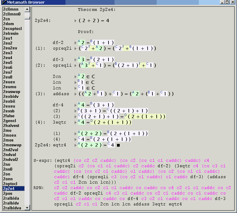